2 Neural Network Properties

   
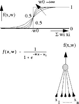
Figure 3: A single neuron (right) and its input-output relation based on a sigmoid function (above)

The feed-forward neural networks that are discussed here are configured by single neurons such as shown in fig  3 . Their inputs are linearly weighted and summed. The result is mapped by a squashing function on the (0,1) interval. Note that for very small weights this function is almost linear and that for very large weights it almost resembles the step function.

   
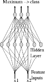
Figure 4: Feedforward network for 2 features and 3 classes

An entire neural network with a single layer of hidden neurons is shown in fig  4 . It has an input for each feature and an output for each class. Classification is done by assigning the label of the class with the highest output to the incoming feature vector. The number of hidden neurons can be freely chosen and determines the maximum nonlinearity that can be reached. Almost any decision surface can be constructed for sufficiently large sets of neurons.

It is important to distinguish the architecture of a neural network from the way it is trained. It has been shown in literature that almost any classifier can be mapped on a neural network. This shows that the architecture is very general and it is thereby not specific. Consequently, from a scientific point of view a neural network implementation of an otherwise trained classifier is thereby not of interest, it does not specifically contribute to a better generalization.

The real interesting point is therefor the way neural networks are trained. If this makes use of the specific architecture, we will call it a neural network classifier. If the training is done otherwise it belongs to the large class of non-neural classifiers and such methods are not considered in this section. Specific neural network training procedures train the network as a whole and iteratively minimize some error criterion based on the network outputs and their targets (derived from the class labels).

Traditionally the MSE criterion is minimized using a gradient descent technique resulting in the well-known error backpropagation training rule. This rule is very slow and only feasible by the heavily improved computer speed in the last decade. Methods that use the second derivative in one way or another (conjugated gradient, Levenberg-Marquardt) can be much faster but might also yield instable results.

A number of observations can be made on the properties of neural network classifiers. They are given here without much argumentation:

1. The backpropagation rule and its derivatives very rarely finds the global minimum. The computational effort as well as the large number of local minima in the error landscape are prohibitive.
2. For almost all networks with more than one or two hidden neurons the global minimum is undesirable as an unrestricted neural network classifier has a too large complexity for most problems.
3. It can thereby be concluded that the traditional neural network classifiers work because of the lousy performance of the backpropagation rule. Put it more friendly: this rule has sufficiently built in regularization possibilities, most prominently its large computer demand resulting in early stopping by an impatient analyst.
4. One of the most important reasons why the optimization of complex nonlinear machines like neural networks works, is due to the tradition of starting with small weights. This corresponds with linear neurons (see fig  3 ) and thereby with an entire linear neural network. Consequently, in the first step an optimal linear solution is approximated, thereafter, due to the growing weights, the network represents a moderate nonlinearity. After that it stops at one of the nearest local minima, see [9] for a more extensive discussion.
5. The above may also be formulated as: a neural network shows an increasing complexity as a function of the training effort. This is illustrated by the behavior of the error as a function of the training time, see fig  5 compared with fig  1 .

      
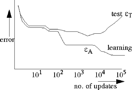
   Figure 5: A neural networks classifier shows increasingly more overtraining for more updates due to an increasing effective classifier complexity
   

6. Faster neural methods have less built in regularization and should therefor be more explicitly protected against overtraining, e.g. by the addition of noise or by weight decay.
7. Most neural networks are redundant: they have more neurons than needed for implementing the final classifier. This redundancy, however, helps during the training procedure.
8. The neural network solution is hardly ever the best classifier for a given problem. However, very often they do reasonably well. It has to be realized that due to the very large set of possible neural network solutions, results highly depend on the skills of the analyst. A unique neural network classifier (like the well defined 1-nearest neighbor rule) does not exist, see [11].