3 Further Observations

One of the most important lessons that can be extracted from the neural network invasion that entered the pattern recognition area is that it appears to be possible to train large, complex machines that often have more degrees of freedom than the size of the training set. The widely accepted dogma, based on the work by Cover, that one should never do this has therefore to be reconsidered.

A simplified version of the traditional argumentation is that a linear classifier in , having k degrees of freedom, is always able to separate perfectly an arbitrarily labeled training set of training samples and has thereby no generalization capability. Computations by Cover [8] and later by Vapnik [4] show that , e.g. n = 10 k , in order to get some generalization. In these studies it is not taken into account that in many applications it is known on apriori grounds that the classes are reasonably well separable. On the same arguments as given for the linear classifier, the more complex and nonlinear neural network classifier should not be used in small sample size situations, but appeared to give good results in practice.

   
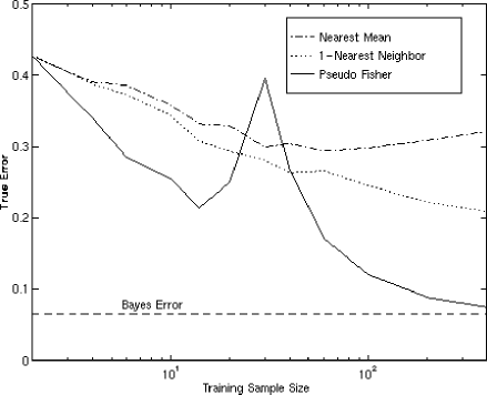
Figure 6: The averaged error (50 runs) of some classifiers for a 30-dimensional Gaussian problem

Stimulated by these observations the first author started to reinvestigate the linear classifier for n < k . One of the first things that could be observed is that an adaptation of the traditional Fisher's Linear Discriminant using a pseudo-inverse technique (the PFLD) yields a surprising result for the separation of two 30-dimensional Gaussian distributions [10], see fig  6 . The mean error peaks for n = k = 30. On the left side of this peak it pays off to throw away a part of the training set at random. If this data set reduction is done more systematically using some heuristic strategy (the Small Sample Size Classifier, SSSC, [10]) an even better result can be obtained. This behavior can be understood by realizing that for n < k the data is situated in a linear subspace, such that there is a preference for directions with large variances. If these directions coincide with the class differences, the additions of more samples, and thereby more feature directions will mainly introduce more noise and will yield

It should be noted that in the step from PFLD to SSSC a shift in criterion has been made. Fisher's discriminant is based on a MSE criterion. In case of the PFLD this criterion is still used but yields a zero MSE as the number of parameters (the feature size) is larger than the sample size. The SSSC now heuristically minimizes the number of objects in the training set under the condition that still a zero MSE is obtained. So this follows a minimum description length (MDL) strategy.

More systematically this is done by a recent proposal by Vapnik [5], the Support Vector Classifier (SVC). If the training set is given by a matrix X the weight vector w for a linear classifier C ( y ) for a new object vector y can be written as a linear combination of the original training set:

The MSE solution of a for a given set of class labels (output targets) is:

so

in which stands for the matrix of inner products between X and Y (or y ). The FLD and the PFLD can be written like this. If n <= k the MSE is zero. In the SVC the training set X is reduced to a minimal set. Vapnik [5] uses a quadratic programming technique which allows also nonzero MSE solutions and thereby training set sizes n > k . He also shows that by replacing K by a polynomial classifier is obtained having the same complexity as the linear one! This is due to the fact that the length of the parameter vector a equals to size of the support set.

In [12] and [13] we proposed to replace the inner product matrix by an arbitrary similarity matrix based on direct measurements of object (dis)similarities, resulting in a featureless approach to pattern recognition. This procedure seems to be a good candidate to meet the challenge presented in the first section: higher image resolutions now result in more accurate computations (of object similarities) only. The classifier itself doesn't change. As a result of the fixed parameter size there are no problems with an increasing complexity.

   
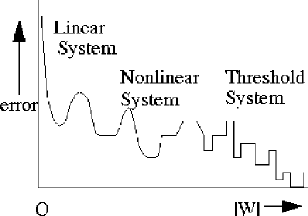
Figure 7: Neural network error behavior as a function of the total weight size

At this point in our discussion we report an interesting perceptron study recently undertaken by Raudys [15]. His aim is to get a better understanding of the neural network learning behavior. In [9] we summarized this using fig  7 . Due to the small weight initialization a neural network starts as a linear system, for growing weights the nonlinear part of the sigmoid function is used, see fig  3 , and for very large weights the sigmoid behaves as a threshold function that just counts the errors. Some of Raudys' observations will now be summarized and commented.

In order to study the linear initialization better, targets of 0.4 and 0.6 are used. Raudys proves formally and experimentally that by this the perceptron has a MSE behavior and approaches Fisher's Linear Discriminant. If the targets are released to extreme values, e.g. 0.001 and 0.999 the outputs are allowed to use the nonlinear part of the sigmoid. As a result a minimum error probability behavior is found for just weakly overlapping classes: the perceptron approaches the linear classifier that minimizes the apparent error.

If training is proceeded further the perceptron becomes insensitive for the most remote objects and training becomes determined by the most nearby objects only. We suggest that if at this point the weights of the most remote objects are set to zero, the perceptron might be used to find a support vector classifier. So now we have a MDL solution. In the next section an experimental examples is given. Raudys concludes that the target value is a very important regularization parameter, in combination with the training time. It has to be studied further how Raudys' results should be extended to the nonlinear case for neural networks with more layers.

A remarkable conclusion can be drawn from Raudys' study. A neural network is not just able to implement almost any classification function, but it can also be trained with various strategies. We add to this conclusion that this neural network ability may only be judged positively if it appears to be possible to formulate explicit rules how this has to be done for an arbitrary problem. Otherwise this neural network ability remains hidden in the skills of the analyst.