


After a candidate kerb has been localised, we can segment the image edge points into three regions: one for the kerb, one for pavement and one for road. Moreover, we would like to determine whether it is a step-up or step-down and estimate its size.
In the x-y coordinate system, for each edge point found by the edge detector, we can compute the distance to the origin of
the line passing through this point and perpendicular to slope
found by the edge detector, we can compute the distance to the origin of
the line passing through this point and perpendicular to slope :
:

We compare the
r
for each point with and
and :
:
If , then the point is classified as belonging to the outside region, for
example, point
, then the point is classified as belonging to the outside region, for
example, point in Figure
2
. If
in Figure
2
. If , then the point is classified as belonging to the inside region, for
example, point
, then the point is classified as belonging to the inside region, for
example, point in Figure
2
. If
in Figure
2
. If , the point is in the kerb region.
We do this for both images, provided that there are sufficiently many features on the ground. We then perform stereo matching and ground-plane fitting in the inside and outside regions individually, finally obstacle detection. The flow diagram in Figure 5 shows the integration of GPOD with kerb detection.
Ā
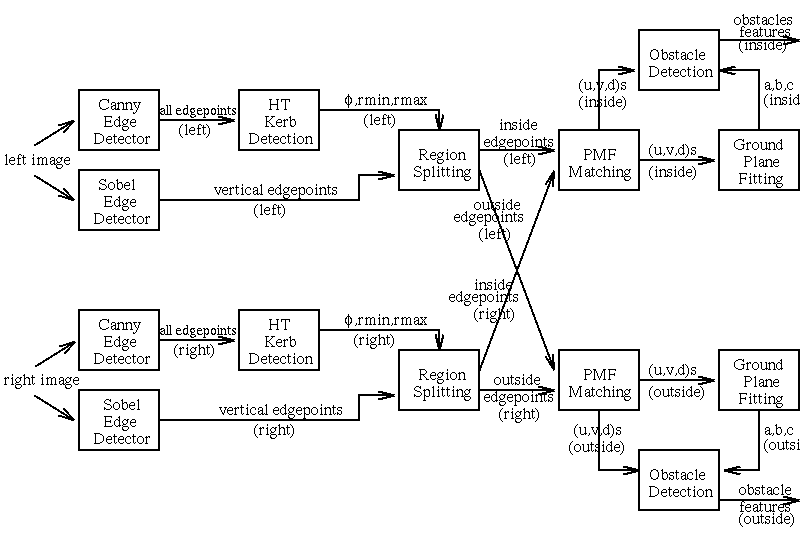
Figure 5:
Flow diagram for the integration of Ground Plane Obstacle Detection and
Kerb Detection
We have


for the estimated kerb position in each image. Averaging between the
left and right images gives the cyclopean kerb position which can be converted to give approximate 3-D range information with
the roughly calibrated camera intrinsic parameters.
which can be converted to give approximate 3-D range information with
the roughly calibrated camera intrinsic parameters.
Let and
and be the ground plane parameters obtained for the inside and outside
regions respectively. We have
be the ground plane parameters obtained for the inside and outside
regions respectively. We have


If , it is a step-down, else it is a step-up.
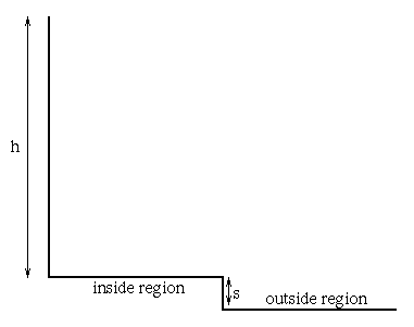
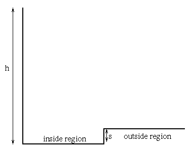
For a step-down of size s as shown in Figure 6 (a), the effect on the ground plane parameters from inside region to outside region is like increasing the height h of the camera system by s . It can be shown [ 11 ] that

Similarly for a step-up case as shown in Figure 6 (b),

Using the error propagation formula for the quotient of two uncorrelated distributions [ 1 ], we have

In this way, not only can we estimate the height of the kerb, but its uncertainty can be computed.
|
|

|

|
Figure
7
shows an 128x128 stereo image pair for an artificial kerb scene. The
kerb is approximately 8cm high and 100cm away from the cameras, which
are 120cm above the ground. We apply the above approach to find the kerb
region in order to segment the image: we find that the estimated kerb
distance is 109cm. Assuming , the ground plane fitting as described in Section
2
gives:
, the ground plane fitting as described in Section
2
gives:
The inside region ground plane parameters are -0.0348, 0.2144 and
33.2667 with variances ,
, and
and respectively. The outside region ground plane parameters are 0.1037,
0.2295 and 20.8608 with variances
respectively. The outside region ground plane parameters are 0.1037,
0.2295 and 20.8608 with variances ,
, and
and respectively. The disparity for the inside kerb region is 44.0466 with
variance 0.7388. The disparity for the outside kerb region is 40.8520
with variance 1.2992. Since the inside disparity is greater than the
outside disparity, it is a step-down: its mean size and standard
deviation are estimated as 9.38cm and 4.41cm respectively.
respectively. The disparity for the inside kerb region is 44.0466 with
variance 0.7388. The disparity for the outside kerb region is 40.8520
with variance 1.2992. Since the inside disparity is greater than the
outside disparity, it is a step-down: its mean size and standard
deviation are estimated as 9.38cm and 4.41cm respectively.

|

|
Figure 8 shows the step-down from another angle, Figure 9 shows the graph for the matched edge points together with the fitted ground plane using all points and the fitted ground planes using just points in the lower or upper region. This is a typical two-population problem and it can be seen that ground-plane fitting the points in each individual region will help in more accurate small obstacle detection.
Ā
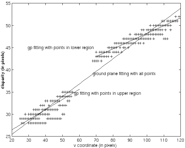
Figure 9:
Ground plane fitting using just points in the lower region, upper region
and whole region
Stephen Se