


Several methods for adapting GAs to cope with the simultaneous optimisation of a problem over a number of dimensions have been proposed, including the use of Pareto-ranking, [10]. The MOGA applied in this work uses Pareto-ranking as a means of comparing solutions across multiple objectives. The Pareto-optimal set of a multiobjective optimisation problem consists of all those vectors for which their components cannot be all simultaneously improved without having a detrimental effect on at least one of the remaining components. This is known as the concept of Pareto optimality [10], and the solution set is known as the Pareto-optimal set (or non-dominated set).
GAs have been recognised to be well-suited to multiobjective optimisation as described in [11] and [12]. MOGAs do not impose an ill-informed weighting process on the task of selecting a single optimal solution but instead the concept of pareto-ranking can be applied in order to deliver a set of candidate solutions optimised for different combinations of criteria.
The advantages of GAs have already been used by computer vision researchers, examples of which are described in [8] and [9]. GAs are particularly applicable to the problem addressed in this paper, as our search space is noisy, discontinuous, impractical to search exhaustively and contains no derivative information. Also the criteria we wish to optimise are interdependant within the definition of the database. Selecting the correct set of histograms to compactly represent a set of objects for the most reliable and unambiguous recognition results is a computationally demanding problem.
To explain the selection of the objective functions for the GA, it is useful to recall the motivation for applying a MOGA: for a given scene or model line we have a choice of the parameters for the associated PGH. Our algorithm will optimise these parameters producing optimal sets of lines relative to all others in the database. In what follows B denotes the Bhattacharyya match score between two histograms and is defined as:

where and
and are two PGHs of the
same type
,
are two PGHs of the
same type
, the number of bins on the
 axis and
 the number of bins on the perpendicular distance axis.
B
is used as a measure of similarity between two histograms - two
identical histograms yield
B
=1 (assuming the histograms are normalised) and two completely
dissimilar histograms give
B
=0.
the number of bins on the perpendicular distance axis.
B
is used as a measure of similarity between two histograms - two
identical histograms yield
B
=1 (assuming the histograms are normalised) and two completely
dissimilar histograms give
B
=0.
Suppose we have a set of PGHs. We require a principled technique for
determining the relative distinctiveness of each of the histograms in
the set. For a given PGH belonging to such a set, this can be achieved
by calculating the match scores between our given PGH and all others in
the set. We seek to maximise the distance between the identical match
B
=1 and the
mean
of all the other matches, as the greater this quantity, the more
distinct our given PGH will tend to be relative to the rest of the set,
hence our first objective, , is:
, is:

In addition, we want a measure that reflects histogram consistency (or line labelling) across different examples of a given object subject to variable segmentation/fragmentation. We will consider different sets of data: variant sets , defined as follows:
 .
.
So for a given histogram this measure will tell us which of the variant sets that particular PGH was most likely to have come from. We can achieve this by calculating the matches between our given histogram and all PGHs in each variant set. The best match between our given PGH and all the PGHs for each object in each variant set is stored (the inner summation of equation 2) and then these best matches are summed for each variant set. The variant set with the highest sum is the winner and the given histogram is deemed to have come from the winning variant set. This avoids the difficult problem of labelling corresponding lines in the database. Thus:

(where is the number of objects in variant set
j
and
N
is the number of variant sets).
is the number of objects in variant set
j
and
N
is the number of variant sets). is potentially computationally intensive, as it involves computing the
matches between all histograms in the variant sets for
every
member of our GA population. Here the ability of the GA to optimise on
stochastic objective functions is of value.
is potentially computationally intensive, as it involves computing the
matches between all histograms in the variant sets for
every
member of our GA population. Here the ability of the GA to optimise on
stochastic objective functions is of value.
Finally we desire as compact a representation as possible and therefore
want to minimise the area of the histograms. For this work the bin width
of the histograms is fixed and the only variable parameters for area are
the perpendicular distance, (which is also the radius of the circular window used for constructing
the PGH), and the histogram type. So the third objective function
minimises the histogram area. A scale factor of 1, 2 and 4 for mirrored,
rotated and directed histograms respectively (FigureĀ
2(a)
) was used reflecting the associated area, (since rotated histograms
have twice the area of mirrored and directed twice the area of rotated).
Hence we have:
(which is also the radius of the circular window used for constructing
the PGH), and the histogram type. So the third objective function
minimises the histogram area. A scale factor of 1, 2 and 4 for mirrored,
rotated and directed histograms respectively (FigureĀ
2(a)
) was used reflecting the associated area, (since rotated histograms
have twice the area of mirrored and directed twice the area of rotated).
Hence we have:

In our encoding scheme an individual is represented as shown in FigureĀ
2(b)
. The HISTOGRAM in the encoding is a PGH constructed from a reference
line belonging to some object in a variant set. The TYPE and
refer to the histogram, being the histogram type and maximum
perpendicular distance respectively.
Ā
Ā
Ā

Figure 2:
Illustration of PGH Types and Encoding Scheme Used
The MOGA population consisted of sub-populations each of which was
stored as an array of individuals. FigureĀ
3
shows pseudo code for the MOGA. The number of individuals in each
sub-population was equal and did not change. Initially the
sub-populations were randomly generated and each individual assigned a
fitness based on its pareto-rank. Fitness was then assigned by taking
the compliment of the pareto-rank with the sub-population size
. By summing the fitness across all individuals within a sub-population
we could assign a fitness for that sub-population. The sub-populations
were then randomly paired for crossover and mutation, producing two new
sub-populations. The individuals in the new sub-populations were
evaluated and similarly the new sub-populations were assigned a fitness.
Initially Stochastic Universal Sampling, ([15]) was used for deciding
which sub-populations to keep, but it was found that a more efficient
technique for selection was simply to compare the fitness of the old
sub-populations (prior to crossover and mutation) and the newly created
sub-populations. If the new sub-population was fitter, it was retained
and the old one discarded (and vice-versa). Finally for each
sub-population the individuals were sorted in descending order according
to their fitness (Grouping() in FigureĀ
3
).
Ā
Ā

Figure 3:
Pseudo Code for MOGA
In order for crossover to function as desired we needed to ensure that two good sub-populations produced fit/fitter offspring sub-populations. Crossover was performed by randomly selecting a pair of sub-populations and two crossover points (corresponding to rows of the arrays). Suppose we had N individuals in each sub-population. Two crossover points were used, the first was N /2 and the second was generated randomly (from the range ( N , N /2)). This was to ensure a balance between randomly crossing and selectively crossing fit groups of individuals.
Ā
Ā

Figure 4:
Crossover Operator Used
Ā
Ā
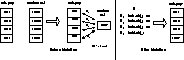
Figure 5:
Mutation Operator Used
Mutation consisted of creating a sup-population of randomly generated individuals and calculating the Bhattacharyya score between each member of that random set with every member of the sub-population (FigureĀ 5 ). For a given individual of the random set, the match score with every member of the sub-population was calculated and if all scores were less than the corresponding individuals fitness on the first objective then the random individual replaces the bottom-most individual in the sub-population (and the replacement continues upwards). This ensures that the population diversity is maintained and that premature convergence did not occur.
Frank Aherne