

Next:
3 Experiments
Up:
Comparison of Combined Shape
Previous:
1 Introduction
Three shape coding techniques are shortly introduced. All of them are
computed from the contour of an object. The object is expected to be the
ordered (
x
,
y
) presentation of the contour pixels.
The chain code histogram (CCH) is meant to group together objects that
look similar to a human observer [
10
]. It is not meant for exact detection and classification tasks. The CCH
is calculated from the chain code presentation of a contour.
The Freeman chain code [
6
] is a compact way to represent a contour of an object. The chain code
is an ordered sequence of
n
links , where
 is a vector connecting neighboring contour pixels. The directions of
 are coded with integer values
k
=0,1,...,
K
-1 in a counterclockwise sense starting from the direction of the
positive
x
-axis. The number of directions
K
takes integer values
 where
M
is a positive integer. The chain codes where
K
>8 are called generalized chain codes [
5
].
The calculation of the chain code histogram is fast and simple. The CCH
is a discrete function
Ā

where is the number of chain code values
k
in a chain code, and
n
is the number of links in a chain code. A simple example is depicted in
Figure
1
. In Figure
1
(a) are the directions of the eight connected chain code. In Figure
1
(b) is a sample object, a square. The starting point for the chain
coding is marked with a black circle, and the chain coding direction is
clockwise. In Figures
1
(c)-(d) are the chain code and the CCH of the contour of the square.
Ā
Ā

Figure 1:
(a) The directions of the eight connected chain code (
K
=8). (b) A sample object, a square, (c) chain code presentation of the
square, and (d) the chain code histogram of the square.
The CCH is a translation and scale invariant shape descriptor. It can be
made invariant to rotations of because the
 rotation causes only a circular shift in the CCH. To achieve better
rotation invariance the normalized chain code histogram (NCCH) should be
used [
10
]. It takes into account the lengths of different directions.
The pairwise geometric histogram (PGH) is a powerful shape descriptor
that is applied to polygonal shapes [
4
,
2
]. It can be applied also to an irregular shape if the shape is first
approximated with a polygon. For a recent review of polygon
approximation algorithms, see for example [
19
].
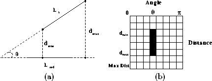
Consider a polygon defined by its edgepoints . Now successive edgepoints define the line segments the polygon
consists of. The PGH is calculated using the following strategy: Let
each line segment be a reference line on its turn. Then the relative
angle
 and the perpendicular minimum and maximum distances (
 and
and ) are calculated between the reference line and all the other lines, as
shown in Figure
2
(a). The histogram values are increased by one on the indexes
corresponding to the angle
 and the line segment from the
 to
to (Figure
2
(b)).
Ā
Ā

Figure 2:
(a) Relative angle and perpendicular distances between two lines, and
(b) the pairwise geometric histogram.
A new scheme to reduce the size of the PGH is proposed. Conditional
expectations of each row and column are calculated and collected into a
feature vector. Let
p
(
i
,
j
) be the PGH value in the position (
i
,
j
). Then the feature vector is given as

where
N
is the number of rows of the PGH,
M
is the number of columns of the PGH, is the conditional expectation of the
i
th row,

and is the conditional expectation of the
j
th column,

Thus the number of features is reduced from
NM
to
N
+
M
. This presents significant savings in calculation time and memory
requirements, especially if
N
and
M
are large.
In this section, five simple shape descriptors are introduced (Figure
3
). Variations of most of them have been widely used in object
recognition [
12
,
17
]. Each descriptor alone is insufficient for a complex recognition task,
but the combination of them is shown to have good recognition
capabilities (Section
3
). All these shape descriptors require only calculation steps expect convexity which requires
 calculation steps. For a more profound discussion and definitions of
these descriptors, see [
15
].
Ā
Ā

Figure 3:
Five simple shape descriptors.
Convexity can be defined as the ratio of perimeters of the convex hull
of the contour and the original contour. The convex hull is the minimal
convex covering of an object. The algorithm for constructing a convex
hull involves traversing the contour and minimizing turn angle in each
step. Practically, dot product can be maximized instead.
Principal axes of an object can be uniquely defined as segments of lines
crossing each other orthogonally in the centroid of the object and
representing the directions with zero cross-correlation. This way, a
contour is seen as an realization of a statistical distribution. The
ratio of principal axis can be calculated from the covariance matrix of
a contour. It is not necessary to calculate actual eigenvectors nor
eigenvalues.
Compactness is often defined as the ratio of squared perimeter and the
area of an object. It reaches the minimum in a circular object and
approaches infinity in thin, complex objects. The measure applied in
this paper is the ratio of the perimeter of a circle with equal area as
the original object and the original perimeter.
Sometimes a shape should be compared against a template. A circle is an
obvious and general template choice. The circular variance is the
proportional mean-squared error with respect to solid circle. It gives
zero for a perfect circle and increases along shape complexity and
elongation.
Elliptic variance is defined similarly to the circular variance. An
ellipse is fitted to the shape (instead of a circle) and the
mean-squared error is measured.


Next:
3 Experiments
Up:
Comparison of Combined Shape
Previous:
1 Introduction
Jukka Iivarinen
Wed Jun 18 13:02:47 EET DST 1997
 , where
 is a vector connecting neighboring contour pixels. The directions of
 are coded with integer values
k
=0,1,...,
K
-1 in a counterclockwise sense starting from the direction of the
positive
x
-axis. The number of directions
K
takes integer values
 where
M
is a positive integer. The chain codes where
K
>8 are called generalized chain codes [
5
].


 is the number of chain code values
k
in a chain code, and
n
is the number of links in a chain code. A simple example is depicted in
Figure
 because the
 . Now successive edgepoints define the line segments the polygon
consists of. The PGH is calculated using the following strategy: Let
each line segment be a reference line on its turn. Then the relative
angle
 and the perpendicular minimum and maximum distances (
 and
and ) are calculated between the reference line and all the other lines, as
shown in Figure
 and the line segment from the
 is given as
 is the conditional expectation of the
i
th row,
 is the conditional expectation of the
j
th column,
 calculation steps expect convexity which requires
 calculation steps. For a more profound discussion and definitions of
these descriptors, see [