


An experiment was conducted to compute the matrix for an echocardiographic data set. The peak of the ECG R-wave was
chosen as the starting point to a cardiac cycle. The first frame of the
image sequence was then manually segmented. The resulting spline, with
14 control points defined the initial template. Four non-consecutive
cycles were selected in this way, with the aim of obtaining a
representative sample of heart cycle variations. Table
1
summarises the results of PCA analysis. For this data set, four modes
explained
matrix for an echocardiographic data set. The peak of the ECG R-wave was
chosen as the starting point to a cardiac cycle. The first frame of the
image sequence was then manually segmented. The resulting spline, with
14 control points defined the initial template. Four non-consecutive
cycles were selected in this way, with the aim of obtaining a
representative sample of heart cycle variations. Table
1
summarises the results of PCA analysis. For this data set, four modes
explained of the variation.
We can express any shape in a training set as an initial template plus a
multiple of the estimated
matrix. As we have seen in the last section we can chose
via principal component analysis, such that the of the variability is explained by the first
k
eigenvalues. (in example 1,
k
=4,
N
=95).
of the variability is explained by the first
k
eigenvalues. (in example 1,
k
=4,
N
=95).
It is possible to take the mean shape and add to it multiples of each mode to see what that particular mode
represents. Equation
1
becomes,
and add to it multiples of each mode to see what that particular mode
represents. Equation
1
becomes,

where, is the
i
th eigenvector,
is the
i
th eigenvector, is the
i
th eigenvalue which represents the sample variance of
is the
i
th eigenvalue which represents the sample variance of , and
m
is a scalar usually varying between 1 and 3.
, and
m
is a scalar usually varying between 1 and 3.
Mode
Eigenvalue
Variability percent
Cumulative variability
1
360197.5
0.712
0.712
2
60381.77
0.119
0.832
3
41323.56
0.0817
0.913
4
21986.23
0.0435
0.957
of the variability.
Plots of the first four modes for this example are shown in Figure
1
(top). The thicker contour is the mean shape curve. The two thinner
curves represent the mean shape standard deviations. The first mode appears to be a translation mode.
The second mode appears to be a scaling mode where the scaling applies
to the bottom of the left ventricle next to the mitral valve. The third
and fourth modes both appear to represent a combination of scaling and
translation.
standard deviations. The first mode appears to be a translation mode.
The second mode appears to be a scaling mode where the scaling applies
to the bottom of the left ventricle next to the mitral valve. The third
and fourth modes both appear to represent a combination of scaling and
translation.
Ā
Ā

Figure 1:
Principal component analysis performed on 4 cardiac cycles of a
ultrasonic image sequence.
Top
: The mean shape (thick curve) is plotted along with curves representing
the addition of
standard deviations to the mean shape mode; From left, mode 1 (the
dominant mode) to mode 4.
Bottom
: The mean shape (filled line) is plotted along with flow lines
representing how the start of each span behaves with the addition of
standard deviations to the mean. From left, mode 1 (the dominant mode)
to mode 4.
An alternative way of visualising the modes of variation is depicted in
Figure
1
(bottom). Here flow vectors have been used to indicate the deformation
for selected points along the contour. In this figure each flow vector
is centred on a point on the mean shape. The ends of the flow vectors
are located at three standard deviations from the mean shape taken in the direction of
the shape deformation. The attraction of this method of visualisation is
that it can be used to highlight the degree of scaling, translation and
rotation for a general shape deformation. This can be difficult to
determine by simply plotting the shape modes (Figure
1
(top). For example, in Figure
1
(bottom) it is clearer now that although mode 1 is predominately a
translation mode there is also a small rotation component. Mode 4 shows
a strong horizontal translation component.
three standard deviations from the mean shape taken in the direction of
the shape deformation. The attraction of this method of visualisation is
that it can be used to highlight the degree of scaling, translation and
rotation for a general shape deformation. This can be difficult to
determine by simply plotting the shape modes (Figure
1
(top). For example, in Figure
1
(bottom) it is clearer now that although mode 1 is predominately a
translation mode there is also a small rotation component. Mode 4 shows
a strong horizontal translation component.
Recall from Equation
1
that the shape-space model is given by,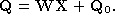
 can be recovered as,
 where
where is the pseudo-inverse of
 . Figure
2
shows plots of the shape-space vector
over time. Note in particular the periodicity of the second mode.
Temporal plots of this kind are potentially of great clinical value for
quantifying heart periodicity and asynchronousy. We plan to investigate
this idea in future work.
. Figure
2
shows plots of the shape-space vector
over time. Note in particular the periodicity of the second mode.
Temporal plots of this kind are potentially of great clinical value for
quantifying heart periodicity and asynchronousy. We plan to investigate
this idea in future work.
Ā
Ā
Figure 2:
Plots of the four components of
over one cardiac cycle; from (a) to (d), components 1 to 4. Each
component is plotted against the time for the image sequence.
Recall from Section 2.1 that it is possible to define the
matrix with varying degrees of freedom (dimensionality). A low
dimensional space, such as an affine space, is attractive as it is
easier to compute and offers an intuitive interpretation. All prior work
on tracking hearts in 2D image sequences has assumed this model. On the
other hand a higher dimensional space might be necessary for accurately
characterising deformation and tracking. An experiment was conducted to
investigate how close a
matrix estimated using PCA and training was to an affine space. The
purpose of this experiment was to see whether a higher dimensional space
was really necessary for characterising heart dynamics.
The residual r defined as,

was used as the similarity metric. Here is an eigenvector of the PCA
matrix,
is an eigenvector of the PCA
matrix, is an affine shape matrix and
 is its corresponding pseudo-inverse.
Eigenvector
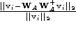


0.3411
0.1163

0.2931
0.0859

0.9392
0.8821

0.4811
0.2315
matrix obtained using PCA into an affine space. Shown is the residual
after projecting into the affine space,
.
Table
2
summarises the residuals computed for the first four modes of the normal
heart image sequence PCA
matrix. This shows that although modes 1,2 and 4 are fairly close to
affine components, only of mode 3 can be explained by an affine deformation. The importance of
this results is that it tells us that the dynamics of the left
ventricular boundary cannot be modelled well by an affine deformation.
of mode 3 can be explained by an affine deformation. The importance of
this results is that it tells us that the dynamics of the left
ventricular boundary cannot be modelled well by an affine deformation.
An alternative way to compare how well different shape-models capture
heart dynamics is to perform a visual inspection of tracking
performance. An experiment was performed to compare tracking results
using (1) a
matrix chosen to correspond to an affine shape matrix, (2) a
matrix estimated using PCA and (3) a
matrix estimated using PCA followed by training.
Figure 3 shows `snapshot' views of tracking using the three approaches on three consecutive frames. The main conclusion that we could draw from this experiment was that tracking based on methods (2) and (3) gives superior results to method (1) in terms of how closely the tracker followed the observed heart chamber boundary movement. This indicates that that heart dynamics are not well modelled by a (simple) affine model. Training - method (3) - did appear to be slightly more resilient to spurious features and was less sensitive to parts of the contour fading out of the measurement window over part of the cardiac cycle. However, this approach is computationally more expensive. It was also very apparent from this study that further improvement in tracking performance could only be achieved by enhancing the image feature detection process. We consider this next.
Ā
Ā
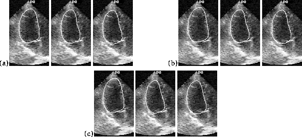
Figure 3:
Echogram tracking using affine W matrix (left), W matrix from PCA
(middle), trained tracker using W matrix from PCA (right). (a) - (c)
Frames 44, 45, and 46.
Gary Jacob