 ), or alternatively, pixels are replaced with a random value in the
range (0,255) with a noise density of 0.2. The resulting images are
clipped into the range (0,255).


Ā Noise interacts with CCD images and photographs in a complicated mannerĀ[ 31 , 32 ]. Furthermore the underlying noiseless image distribution is also extremely complicated. For this reason it is usual to study the performance of filters using rather stylised models of images and noise. Here we shall consider the underlying image to be a disc or a square which we shall assume is corrupted with either Gaussian noise (a model of noise in the imaging system) or impulsive noise (a model for specular reflection or pixel drop-out).
FigureĀ
4
shows examples of the target images. The target image is a disc or
square of amplitude 144 in the centre of a 100 by 100 pixel image with
background 112. To this, is added either uncorrelated Gaussian noise ( ), or alternatively, pixels are replaced with a random value in the
range (0,255) with a noise density of 0.2. The resulting images are
clipped into the range (0,255).
Ā
Ā

Figure 4:
Examples of noise-corrupted images: Gaussian noise (left) and Impulsive
noise (right)
The performance of sieves is compared to Gaussian processors in which the scale-space was generated using separable filters where the image at scale s is computed as in ( 2 ). The scale-selection surface ([ 5 ] p. 323)
is used to locate the scale-space estimate of the target parameters (its scale, ( s ) and position, ( x , y )). For the sieve the scale-selection surface is formed from the granule functions. In the absence of noise both scale-selection surfaces will have a peak corresponding to the target.
An iterative search is conducted over all scales to find this maximum. The linear scale-space processor is scale-calibrated by normalising s so that the peak in ( 7 ) corresponds to the true area of the disc. Improved precision position estimates are obtained through least-squares interpolation around the scale-selection surface peak. Since the area sieve operates by ``slicing off'' peaks and troughs, the extrema may be large and flat so the centroid of these is taken as the position estimate.
| cc | diff | m | M | N | O | ||
| Gaussian |

|
0.212 | 0.643 | 0.280 | 0.241 | 0.261 | 2.882 |
| noise |

|
0.198 | 0.629 | 0.243 | 0.244 | 0.251 | 1.141 |

|
30.30 | 32.4 | 55.0 | 58.9 | 48.7 | 105.75 | |
| Impulsive |

|
0.273 | 0.925 | 0.0425 | 0.0464 | 0.0400 | 0.076 |
| noise |

|
0.330 | 0.790 | 0.0416 | 0.0382 | 0.0448 | 0.712 |

|
35.85 | 59.9 | 3.91 | 3.90 | 4.30 | 8.894 |
Table 1 shows that, in Gaussian noise, the diffusion system,
M
-,
N
-, and
m
-sieves approach the performance of the benchmark normalised
cross-correlation system in which a series of increasing scale target
templates are used. Opening- or
O
-sieves, in which one repeatedly applies increasing scale greyscale
openings, have worse performance (it is known that openings are
sensitive to noise). The result of multiscale closing is not shown since
the closing operator cannot resolve a positive disc under these
conditions
 . Studies with the equivalent one-dimensional filtersĀ[
33
] showed that the linear diffusion system is more sensitive to Gaussian
noise than the sieve. In two-dimensions this is not the case, probably
because the diffusion filter matches the shape of the target. For square
or rectangular targets the diffusion system does not perform so well.
Table 1 also shows the results of the impulsive noise tests. The m -, M -, N - and O -sieves can produce better scale and position estimates than those from the diffusion system. This is an important property since in real vision systems impulses, glint and occlusion are commonplace. Again, the asymmetry of multiscale closings means that the experiment would have to be specially tuned to handle positive targets.
Ā
Ā

Figure 5:
Variation in scale estimates for images with increasing target
amplitude. Gaussian noise tests on the left, impulsive noise tests on
the right. Diffusion results are shown as a solid line, sieve results as
a dashed line.
The performance of sieves in replacement noise is not surprising since
it is known that, in one dimension, and
and filters behave similarly to median filters which have good performance
in impulsive noise. The sieve retains its performance in Gaussian noise
because the cascaded operation described in (
5
) means that, like wavelets, the output at large scales has a large
support.
FigureĀ 5 shows the variation in scale estimates caused by changing the signal-to-noise ratio of the images. This is achieved by altering the target disc intensity. In Gaussian noise, for small intensity targets, the diffusion processor is superior to the m -sieve. As the intensity of the disc increases the performance of the sieve improves, approaching that of the diffusion processor. For discs corrupted with impulsive noise the target amplitude does not alter the sieve's performance. The noise is localised to one scale and is easily removed and although the performance of the diffusion processor improves with increasing disc amplitude, the sieve remains superior.
Why is the performance of image processors in noise important? Studies of imaging noise in general purpose CCD images and photographs show that the noise model is complicated with a Gaussian pdf in which the parameters of the pdf depend on the image intensity but that, for most images, the noise level is low. We believe it is the impulsive noise model that is the most interesting since it forms the basis for a study of occlusion - an important reality that is considered now.
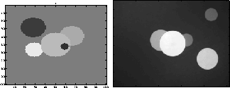
Synthetic test images, for example on the left of FigureĀ 6 , are generated by placing discs of differing area onto a background of amplitude 32. Each 100 by 100 pixel image contains five discs. The target is the only constant image feature. It has an area of 901 pixels and an amplitude of 47. The four occluding discs, areas 49, 253, 481 and 709 pixels, are selected at random (with replacement). They are placed at random, have random intensity (uniform range 0 to 255) and randomly occlude one another. The right-hand side of FigureĀ 6 shows an example real cluttered image with five cardboard discs.
Ā
Ā

Figure 6:
Occlusion image. On the left a synthetic image and on the right a real
image.
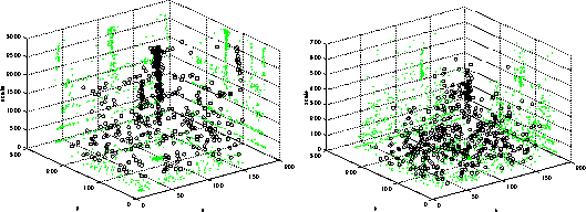
Were the five objects not to have occluded one another, the sieve would produce five granules at the true positions of the objects in scale and space. With occlusion the estimates are degraded. One may judge the degradation by generating test images and plotting granule positions as a function of scale. Results for 100 real cluttered images are shown on the left-hand side of FigureĀ 7 . In FigureĀ 7 the estimates are plotted as circles and their projections on the position and scale planes are plotted as grey dots. For the sieve results the grey dots show a clustering. There are bands corresponding to the scales of the occluding objects and there is a cluster at the centre corresponding to the target.
Repeating this experiment using a diffusion system is more complicated. Extrema must be tracked through scale-space and insignificant extrema due to finite precision effects need to be distinguished from genuine ones. Objects are denoted by maxima along the scale-space tracks.
The right-hand side of FigureĀ 7 shows the result of performing this scale-space tracking on the 100 real images and plotting the maxima on three-dimensional plot as before.
Ā
Ā

Figure 7:
Scale-space estimates for real occluded images. Sieve results on the
left, diffusion results on the right.
The results from the diffusion system are very confused. There is a cluster of points at large scale, corresponding to the target disc. However, at smaller scales very little structure is apparent. Similar experiments using synthetic images show the relative performance of the two systems to be the same.


A. Bosson ESE PG