3 Sieves and their properties

  The basis of the sieve is the representation of an image as a graph [ 27 , 28 ] G = ( V , E ). The set of edges E describes the adjacency of the pixels (which are the vertices V ). For a one-dimensional image the graph is just a list [ 29 ] but for a multidimensional image the graph defines the neighbourhood of a particular pixel. For example, in Figure  2 which shows a four-connected two-dimensional image the graph would be G = ( V , E ) with and . In Figure  2 the numbers are labels not intensities.

   
Figure 2: An image represented as a graph.

The algorithm proceeds by defining a region, over the graph that encloses the pixel (vertex) x ,

where is the set of connected subsets of G with s elements. Thus is the set of connected subsets of s elements that contain x . In Figure  2 , for example, . For each integer the operators , , , are defined as

is a greyscale opening followed by a closing defined over a region of size s and is a greyscale closing followed by an opening over the same region. , .

The types of sieve known as M - or N -sieve are formed by repeated operation of the or operators. They are also known as connected alternating sequential filters. An M -sieve of f is the sequence given by

The N -sieve is defined similarly. The output of an area sieve is usually taken to be the set of granule functions

These form the scale selection surface and non-zero connected regions within granule functions are called granules. Each granule has sharp edges and, at a particular scale, all granules have the same area. In this sense the sieve is scale calibrated , a characteristic illustrated in Figure  1 , that addresses Problem  3 in Section  1 .

   
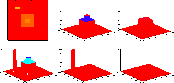
Figure 3: Operation of the area sieve. Original image (left column). Filtered to scale 33 (top centre). Filtered to scale 121 (top right). Granules are shown in bottom centre and right.

An example of the operation of the area sieve is shown in Figure  3 . The figures in the first column show the original 100 by 100 pixel image and its three dimensional intensity plot. The image has one maxima of area 33 pixels on the left-hand side and another of area 121 pixels in the centre. The middle column of Figure  3 shows the result of applying an M -sieve to scale 33 (filtering to scales smaller than 33 pixels produces no change). In the filter output, shown on the top row, the 33 pixel extremum has been removed from the image and is shown as a granule in the granularity domain below. Filtering to increasing scales produces no change up to scale 121 (right column), when the centre extremum is removed. Again this is shown as a granule below. At scale 900 (not shown) the new extremum in the centre of the image is removed leaving a zero intensity image.

The M operation depicted in Figure  3 is the same as the removal of maxima followed by the removal of minima. In an N -sieve these operations are reversed. With this in mind it is possible to define an m -sieve in which the extrema are processed in the order in which they occur as the graph is parsed. In one-dimension such an algorithm is equivalent to the recursive median operator. The m -sieve has properties similar to M - and N -sieves and so not all sieves are alternating sequential filters and not all alternating sequential filters are sieves.

It might appear that the sieving operation could be computationally expensive. In practice, however, the algorithms referred to here, in which the image graph is rewritten as flat-zones are merged, produce scale-spaces much quicker than linear diffusion. Typically a 512 by 512 image is processed in seconds [ 30 , 22 ]. This addresses Problem  4 in Section  1 .

Sieves applied in two-dimensions preserve scale-space causality and this has been proved formally (Theorem 6.36 in [ 22 ]) together with a number of other properties of area sieves (Theorem 6.49 in [ 22 ]). This addresses Problem  2 in Section  1 .

An important property of sieves is that they are invertible  [ 22 ]. Therefore all information in the original image is also available in the granularity domain. Filtering in the granularity domain, followed by a reverse transform (summing all granules), yields a simplified version of the original image.

The properties described so far would appear to be desirable. However, it is well known that morphological operators such as erosion and dilation are sensitive to noise, more complicated morphological filters are less so, and Gaussian filters, having the form of matched filters, are fairly insensitive to noise. Whether sieves, and other filters in their class, have practical application depends on whether they reject image corruptions robustly.