


Separating a combined appearance model into a part that deals with ID
and a part that deals with residual variation allows classification of
ID independently of confounding factors. It also has potential for
applications in model-based tracking of faces. Intuitively, we can
imagine different dynamic models for each separate source of
variability. In particular, given a sequence of images of the same
person we expect the identity to remain constant, whilst lighting, pose
and expression vary each with its own dynamics.
In practise, the separation between the different types of variation
which can be achieved using LDA is not perfect. The method provides a
good first-order approximation, but, in reality, the within-class spread
takes a different shape for each. When viewed
for each individual at a time
, there is typically correlation between the identity parameters and the
residual parameters, even though for the data
as a whole
, the correlation is minimised.
For example, we can reason that the correlation between pose and
identity must be class specific because of the 3D structure of the head;
the way in which the appearance of the nose changes with pose, depends
partly on its length - a person-specific quantity, not derivable from a
frontal view. Ezzat and Poggio [
5
] describe class-specific normalisation of pose using multiple views of
the same person, demonstrating the feasibility of a linear approach.
They assume that different views of each individual are available in
advance - here, we make no such assumption. We show that the estimation
of class-specific variation can be integrated with tracking to make
optimal use of both prior and new information in estimating ID and
achieving robust tracking.
Ā
We describe in a class-specific linear correction to the result of the
global LDA, given new examples of a face. To illustrate the problem, we
consider a simplified synthetic situation in which appearance is
described in some 2-dimensional space as shown in figure
4
. We imagine a large number of representative training examples for two
individuals, person X and person Y projected into this space. The
optimum direction of group separation, , and the direction of residual variation
 , are shown.
Ā
Ā

Figure 4:
Limitation of Linear Discriminant Analysis: Best identification possible
for single example, Z, is the projection, A. But if Z is an individual
who behaves like X or Y, the optimum projections should be C or B
respectively.
A perfect discriminant analysis of identity would allow two faces of
different pose, lighting and expression to be normalised to a reference
view, and thus the identity compared. It is clear from the diagram that
an orthogonal projection onto the identity subspace is not ideal for
either person X or person Y. Given a fully representative set of
training images for X and Y, we could work out in advance the ideal
projection. We do not however, wish (or need) to restrict ourselves to
acquiring training data in advance. If we wish to identify an example of
person Z, for whom we have only one example image, the best estimate
possible is the orthogonal projection, A, since we cannot know from a
single example whether Z behaves like X (in which case C would be the
correct identity) or like Y (when B would be correct) or indeed,
neither. The discriminant analysis produces only a first order
approximation of class-specific variation.
In our approach we seek to calculate class-specific corrections from
image sequences. The framework used is the Combined Appearance Model, in
which faces are represented by a parameter vector , as in Equation
1
.
, as in Equation
1
.
LDA is applied to obtain a first order global approximation of the
linear variation describing identity, given by an identity vector,
, and the residual linear variation, given by a vector
. A vector of appearance parameters,
can thus be described by
where and
and are matrices of orthogonal eigenvectors describing identity and residual
variation respectively.
and
are orthogonal with respect to each other and the dimensions of
and
sum to the dimension of
. The projection from a vector,
onto
and
is given by
are matrices of orthogonal eigenvectors describing identity and residual
variation respectively.
and
are orthogonal with respect to each other and the dimensions of
and
sum to the dimension of
. The projection from a vector,
onto
and
is given by
and
Equation
6
gives the orthogonal projection onto the identity subspace,
, the best classification available given a single example. We assume
that this projection is not ideal, since it is not class-specific. Given
further examples, in particular, from a sequence, we seek to apply a
class-specific correction to this projection. It is assumed that the
correction of identity required has a linear relationship with the
residual parameters, but that this relationship is different for each
individual.
Formally, if
 is the true projection onto the identity subspace,
is the orthogonal projection,
is the projection onto the residual subspace, and
is the true projection onto the identity subspace,
is the orthogonal projection,
is the projection onto the residual subspace, and is the mean of the residual subspace (average lighting,pose,expression)
then,
is the mean of the residual subspace (average lighting,pose,expression)
then,
where is a matrix giving the correction of the identity, given the residual
parameters. If
is an p by 1 column vector, and
an q by 1 column vector, then the matrix
is p by q.
is a matrix giving the correction of the identity, given the residual
parameters. If
is an p by 1 column vector, and
an q by 1 column vector, then the matrix
is p by q.
During a sequence, many examples
of the same face
are seen. We can use these examples to solve Equation
8
in a least-squares sense for the matrix
, thus giving the class-specific correction required for the particular
individual. The vector is unknown, but if we assume that the residual correction is linear,
then
can be found by normalising
and
about the local means of the sequence,
is unknown, but if we assume that the residual correction is linear,
then
can be found by normalising
and
about the local means of the sequence, , and
, and , writing
and
Let represent the elements of
The elements of
represent the elements of
The elements of and
and are independent and the value of the
i
th element of
is given by
are independent and the value of the
i
th element of
is given by
Thus, each row of
relates the residual variation,
, to one of the identity parameters, . If we have
N
>
q
examples of the individual face, we can solve for each row, i, of the
correction matrix separately. Let
. If we have
N
>
q
examples of the individual face, we can solve for each row, i, of the
correction matrix separately. Let be a vector of the examples of
seen and
be a vector of the examples of
seen and a matrix of the examples of
 seen. Let
 be row
i
of the correction matrix, then we can write,
be row
i
of the correction matrix, then we can write,
This is simply an overdetermined system of linear equations and can be
solved for the elements of
by standard methods. Having found
, we can, given a new example, with measured identity,
, and residual variation,
, solve Equation
8
to find
, the corrected identity.
Each column of
describes the effect of each residual parameter on the correction of
identity. The magnitude of the column is a measure of how much new
information has been learnt about the corresponding residual parameter.
For example, if there is very little lighting change in the sequence,
those residual parameters corresponding to lighting will have little
effect on the correction, and the estimate will revert to the orthogonal
projection in that direction.
In each frame of an image sequence, an Active Shape Model can be used to
locate the face. The iterative search procedure returns a set of shape
parameters describing the best match found of the model to the data. We
can also extract the shape-free grey-level parameters from the extracted
shape, and thence calculate the combined appearance model parameters.
Baumberg [
1
] has described a Kalman filter framework used as a optimal recursive
estimator of shape from sequences using an Active Shape Model. In order
to improve tracking robustness, we propose a similar scheme, based on
the decoupling of identity variation from residual variation.
The combined model parameters are projected into the the identity and
residual subspaces by Equations
6
and
7
. At each frame, t, the identity vector,
 , and residual vector
are recorded. Until enough frames have been recorded to allow Equation
13
to be solved, the correction matrix,
is set to contain all zeros, so that the corrected estimate of identity,
is the same as the orthogonally projected estimate,
. Once Equation
13
can be solved, the identity estimate starts to be corrected.
, and residual vector
are recorded. Until enough frames have been recorded to allow Equation
13
to be solved, the correction matrix,
is set to contain all zeros, so that the corrected estimate of identity,
is the same as the orthogonally projected estimate,
. Once Equation
13
can be solved, the identity estimate starts to be corrected.
Two sets of Kalman filters are used, one for the corrected identity
parameters, in which the underlying model of motion is treated as a
zeroth order, or constant position model, and another for the residual
parameters, where the motion model is assumed to be first order, or
constant velocity. This models the sequence realistically during
tracking since the system model treats identity as fixed - something
which is certainly true for sequences - and thus the tracking is robust
to any noise in the tracking corresponding to apparent change of
identity.
Ā
We present an example of this system applied to a face sequence. Figure
5
shows frames selected from a sequence, together with the result of the
Kalman filter-based Active Shape Model search overlayed on the image.
The filter tracks identity as a zeroth order process and residual
variation as a first order process. The subject talks and moves while
varying expression. The amount of movement increases towards the end of
the sequence.
Ā
Ā

Figure 5:
Tracking and identifying a face.
Figure
6
shows the values of the first 3 elements of the corrected identity
vector, . Also shown are similar results without the class specific correction
applied.
. Also shown are similar results without the class specific correction
applied.
It can be seen that the corrected, filtered identity parameters are much more stable than the raw parameters.
Ā
Ā
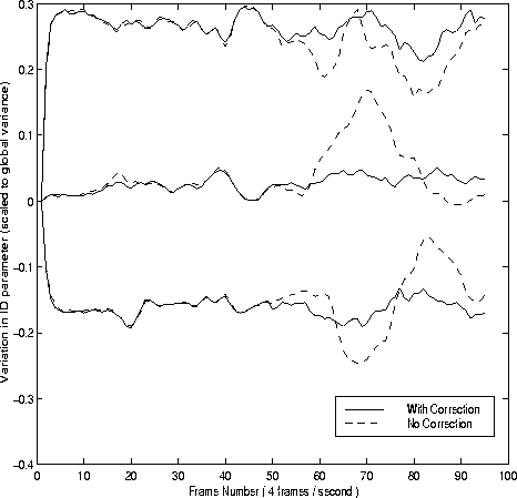
Figure 6:
First 3 parameters of corrected and uncorrected identity vectors.
Parameters are scaled by their respective variance over the training
set.
Gareth J Edwards


