This section describes a correspondence algorithm which produces a
mapping between two triangulated surfaces and
and . In our case, the 3D surface is defined as a set of planar contours.
Each contour represents the outline of a 3D object as it appears in a
single 2D slice of a 3D image. The vertices of these contours are the
pointsets
. In our case, the 3D surface is defined as a set of planar contours.
Each contour represents the outline of a 3D object as it appears in a
single 2D slice of a 3D image. The vertices of these contours are the
pointsets and
and . The connectivity of each pointset is generated from its contour
representation using the algorithm of Geiger [
5
]. This produces densely triangulated polyhedral surface
representations. We assume that the geometric information of each
surface has been normalised such that the centre-of-gravity is at the
origin and the mean distance of the points from the origin is 1. The
output of the algorithm is a pair of sparse polyhedrons
. The connectivity of each pointset is generated from its contour
representation using the algorithm of Geiger [
5
]. This produces densely triangulated polyhedral surface
representations. We assume that the geometric information of each
surface has been normalised such that the centre-of-gravity is at the
origin and the mean distance of the points from the origin is 1. The
output of the algorithm is a pair of sparse polyhedrons and
and for which
 and
and . Pairs of labelled vertices from these polyhedrons comprise a set of
 correspondences. The connectivity of each of the corresponding polyhedra
is identical. The pair-wise correspondence algorithm comprises two
stages:
correspondences. The connectivity of each of the corresponding polyhedra
is identical. The pair-wise correspondence algorithm comprises two
stages:
and
, and
and by triangle decimation; for which
 and
and . The connectivity descriptions of vertices in these polyhedra are
updated during the decimation process. This reduces the computational
complexity of the correspondence task. No correspondences are
established between the pair of shapes at this stage, and the
polyhedrons will usually have a different number of vertices i.e.
. The connectivity descriptions of vertices in these polyhedra are
updated during the decimation process. This reduces the computational
complexity of the correspondence task. No correspondences are
established between the pair of shapes at this stage, and the
polyhedrons will usually have a different number of vertices i.e. .
and
. This is accomplished using a global Euclidean measure of similarity
between both the sparse polyhedron
and a subset of labelled vertices from
and between
and a subset from
. The connectivity and number of vertices from either
or
is chosen to define the polyhedra
and
from the labelled vertices
.
and
. This is accomplished using a global Euclidean measure of similarity
between both the sparse polyhedron
and a subset of labelled vertices from
and between
and a subset from
. The connectivity and number of vertices from either
or
is chosen to define the polyhedra
and
from the labelled vertices and
and .
.
To generate a sparse polyhedron
representing
, we have used a modified version of the triangle mesh decimation
algorithm of Schroeder
et al
[
10
]. The original decimation algorithm had three stages:
 based upon a distance metric
 appropriate to its classification. If
 where
where is some target distance, then the vertex is removed.
Our adaptation of this algorithm makes use of a volume metric rather than a distance metric for the decimation criterion. This is analogous to the area metric of the Critical Point Detection (CPD) [ 15 ] algorithm used for the decimation of polygons in the 2D version of this landmarking framework. The use of a volume metric allows us to treat all of the vertices of a mesh uniformly and to dispense with the vertex characterisation step of the algorithm. As a consequence of this, we may also dispense with the definition of a threshold feature angle.
The volume metric is computed using Schroeder's distance to mean plane
measure. The mean plane associated with a vertex is defined by a unit normal
 and weighted centroid
 which are defined using the
 triangles connected to
:
triangles connected to
:

where ,
, and
and are respectively the centroids, unit surface normals and areas of
triangle
are respectively the centroids, unit surface normals and areas of
triangle connected to
. The volume metric is computed as:
connected to
. The volume metric is computed as:
where and
and are the sums of the areas of the triangles in the loop before and after
decimation respectively, and
are the sums of the areas of the triangles in the loop before and after
decimation respectively, and and
and are the
signed
distances of the vertex
are the
signed
distances of the vertex to the mean plane of the loop before and after decimation i.e.
 . By decimation it is meant that the vertex associated with the loop has
been removed and the resulting hole re-triangulated. Re-triangulation of
the hole is by a recursive loop-splitting algorithm which seeks to fill
the hole with triangles of high aspect ratio.
. By decimation it is meant that the vertex associated with the loop has
been removed and the resulting hole re-triangulated. Re-triangulation of
the hole is by a recursive loop-splitting algorithm which seeks to fill
the hole with triangles of high aspect ratio.
The decimation algorithm is implemented by keeping a list of vertices
sorted by increasing . The head of this list is iteratively decimated and the list updated
until a target number of vertices for the sparse polyhedron is met.
Again, this is analogous to the CPD algorithm used for polygon
decimation. Thus, a sparse polyhedral approximation to our original
triangulated mesh is produced which consists of a subset of vertices of
that mesh, see FigureĀ1.
. The head of this list is iteratively decimated and the list updated
until a target number of vertices for the sparse polyhedron is met.
Again, this is analogous to the CPD algorithm used for polygon
decimation. Thus, a sparse polyhedral approximation to our original
triangulated mesh is produced which consists of a subset of vertices of
that mesh, see FigureĀ1.
Ā
Ā

Figure 1:
Result of applying the decimation algorithm to a triangulated surface of
the left ventricle of the brain. On the left is a shaded representation
of the original dense triangulation with approximately 2000 vertices. On
the right the same surface decimated by 90%.
This stage of the algorithm introduces the only control parameter in the algorithm - the target number of vertices that should be left in the sparse polyhedral representation after decimation. We have determined empirically that the removal of 90% of the original vertices gives an adequate shape representation whilst decreasing the computational cost of finding correspondences and merging shapes in the subsequent stages of the algorithm.
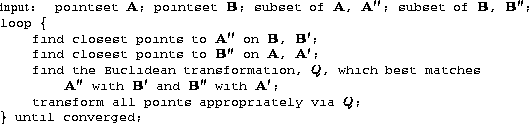
We have used the Iterative Closest Point (ICP) algorithm described by
Besl and McKay [
2
] to establish correspondences between the vertices of
and
. The ICP algorithm determines the Euclidean transformation required to
map one pointset onto another pointset without any initial
correspondence information. We have used a
symmetric
version of this algorithm to establish correspondences of the sparse
pointset with the dense pointset
 and of the sparse pointset
 with the dense pointset
 . Producing correspondences using the sparse polyhedra which have been
generated by decimation cuts down the computational cost of this stage
of the algorithm. The symmetric ICP algorithm is as follows:
. Producing correspondences using the sparse polyhedra which have been
generated by decimation cuts down the computational cost of this stage
of the algorithm. The symmetric ICP algorithm is as follows:
The pointsets
and
are the vertices of the original densely triangulated surfaces, the
subsets
and
are the vertices of the decimated surfaces. An initial estimate of the
pose
Q
is made by finding the translation required to register the centroids of
the pointsets in an intermediate frame, and the scaling required to
equalise the average chord length (average distance from all points to
centroid) of the two pointsets.
Various metrics can be used to define the best match between pointsets. We have used a symmetric measurement of the distance error in registration of the pointsets. We minimise this error such that the pose Q which satisfies:

is determined, where
Q
represents the Euclidean transformation , s is a scale factor,
 is a rotation matrix and
 is a translation. This measures the point registration errors in an
intermediate frame rather than in either frame
is a translation. This measures the point registration errors in an
intermediate frame rather than in either frame or frame
 .
.
The connectivity of the polyhedra may be used to improve the performance
of the algorithm by using information about the surface normals at each
point. We weight the squared distance between points by a factor of
 where
where is the unit surface normal on
 at point
i
, to encourage the correspondence of points on the surfaces which are
topologically equivalent.
at point
i
, to encourage the correspondence of points on the surfaces which are
topologically equivalent.
A single corresponding pair of sparse polyhedra must now be established
from the two polyhedron/pointset pairs, and
and . The choice of connectivity is not critical and so we choose the
connectivity of
(the binary tree framework causes the error of the match to be tested
for both pair orderings). This choice defines one of the corresponding
sparse polyhedra
. The choice of connectivity is not critical and so we choose the
connectivity of
(the binary tree framework causes the error of the match to be tested
for both pair orderings). This choice defines one of the corresponding
sparse polyhedra . The connectivity description of
is now combined with the pointset
. The connectivity description of
is now combined with the pointset to produce a pair of matching polyhedra with a one-to-one mapping
 . The number of correspondences
has now been determined:
. The number of correspondences
has now been determined: .
.
Alan Brett