 at point
 in a distribution by summing the contribution from a mixture of
m
Gaussians:


In the example used above we searched in one image for points similar to the one selected from a second image. For some choices of point in the second image (eg points on the cheeks) we would have many possible matches in the first image. In order to simplify the process of establishing correspondences we would like to try and find matches between the most distinctive points.
Distinct points are those which are least likely to be confused with any other points during a search. Ideally we would like to choose points which occur exactly once in each image we wish to search. As a step towards this we show how to find those points in a single image which are significantly different from all other points in that image.
For every pixel in the image we construct several vectors of invariants, one at each of a range of scales. The full set of vectors forms a multi-variate distribution. If we can model this distribution, we can use it to estimate how likely a given point is to be confused with other points. Distinctive points correspond to vectors which lie in low density regions of the space. In the following we describe how to approximate the distribution and show examples of distinctive points determined by the approach.
We estimate the local density at point
 in a distribution by summing the contribution from a mixture of
m
Gaussians:

We have tried three methods for choosing the parameters.
 ,
, and
and where
N
is the number of samples in the distribution, S is the covariance of the
whole distribution and
h
is a scaling factor. Silverman [
3
] suggests a value for
h
given by:
where D is the number of dimensions. This method gives good results but
its complexity is of order .
.
 of the original
n
points. (
3
) suggests
h
increases as
 decreases. Evaluation of the probability density function is order
 , so can be much more efficient than the kernel method, but this comes
with some loss of accuracy.
The last two methods allow the number of Gaussians used to be specified, which means the execution time can be controlled.
The density estimate for each vector of invariants corresponds directly to the distinctiveness of the pixel at scale
 . The lower the density, the more distinctive the point. A
distinctiveness image can be constructed by setting each pixel to the
density of the corresponding vector at the most distinctive scale for
that pixel. The most distinctive points are then found by locating the
lowest troughs in the distinctiveness image. A scale image can be
constructed by plotting the most distinctive scale at each pixel. This
shows the scale at which each region of the image is most distinct. An
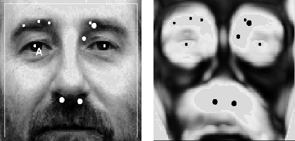
example of locating distinctive points is shown in FiguresĀ
5
,
6
and
6
. FigureĀ
6
is the distinctiveness image obtained from the image in FigureĀ
5
using the Sub-sampled Kernel method with 50 Gaussians. The bright
regions are the most distinct. FigureĀ
6
is the corresponding scale image. The peaks of the distinctiveness image
are superimposed on the original image. The size of the points indicate
the scale at which the points are distinctive.
Ā
Ā
Ā
Ā

Figure:
Distinctiveness image calculated from FigureĀ
5
.
Figure 5:
Original image showing some of the most distinctive points.
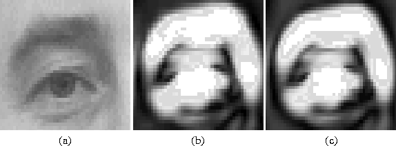
The choice of density estimation method will affect the results. In FigureĀ 7 we compare the distinctiveness images obtained using the Kernel method and the Sub-sampled Kernel method with 50 Gaussians. It can be seen that the Sub-sampled Kernel method provides a good approximation to the Kernel method.
Ā
Ā

Figure 7:
(b) is the distinctiveness image of (a) obtained using the Sub-sampled
Kernel method and (c) uses the Kernel method.
When locating globally distinctive points the finer scales should be ignored because the coarse scale features tend to be the most stable across a set of similar images. For example, human faces have common coarse scale features such as eyes which always look similar, but fine scale features such as wrinkles tend to vary significantly between individuals. Also the coarse scales are less susceptible to image noise. The finer scale features could be used to locally refine an approximate match made by a coarse scale distinct point, but this beyond the scope of this paper.


Kevin Walker