Table 1: Algorithm parameters used in the two experiments


Rigid part segmentation results are presented in this section for 2 sets of range data acquired using a laser striper. For both experiments the same algorithm parameters have been used. These are detailed in Table 1.
Ā
Ā

Table 1:
Algorithm parameters used in the two experiments
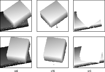
Figure 1 (a) presents a pair of range images each of which contains 2 rigid subcomponents. The subcomponents are simple metallic blocks with planar surfaces. The top figure depicts the components in their original position and bottom figure depicts the components after they have undergone a relative transformation. The dimensions of these range images are 165x182 pixels and 152x175 pixels respectively.
Ā
Ā

Figure 1:
(a) The range images used in experiment 1. (b) The surface patches
segmented from the range images on the first pass of the algorithm. (c)
The surface patches segmented on the second pass.
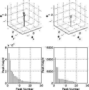
The first pass of the rigid part segmentation algorithm took 213 seconds on a 200MHz Ultra Sparc for this data set. Figure 2 presents details of the rotation Hough transform. The lower of the 2 charts on the left presents the heights of each of the peaks detected in the rotation space in order of importance. The upper of these charts presents the positions in the rotation parameter space of the largest two peaks. The segmentation of the range data based on the largest of these peaks is presented in Figure 1 (b).
Ā
Ā

Figure:
Details of the rotation hough transform constructed for the range data
in Figure
1
. The graphs on the left show the position of the first two peaks (top)
and the height of all of the peaks found in order of significance
(bottom) after the first pass of the algorithm. The graphs on the right
show the peaks details after the second pass.
Having removed the first rigid subcomponent the segmentation algorithm was run again with the remaining range data, this time taking 74 seconds. The details of the rotation Hough transform peak for this pass are presented in the right charts in Figure 2 . The height of this peak is now significantly smaller than in the first pass as much of the spurious Hough transform voting has been removed. The position of this peak has also moved, and is likely to give a better estimate of the second alignment transformation. The segmentation of the range data based on the largest of the new peaks is presented in Figure 1 (c). No surface patches are left at this stage so the segmentation is terminated.
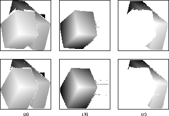
Figure 3 (a) presents a pair of range images each of which contains 2 rigid subcomponents. The top figure depicts the components in their original position and the bottom figure depicts the components after they have undergone a relative transformation. The dimensions of these range images are 181x174 pixels and 184x177 pixels respectively.
Ā
Ā

Figure 3:
(a) The range images used in experiment 2. (b) The surface patches
segmented from the range images on the first pass of the algorithm. (c)
The surface patches segmented on the second pass.
The first pass of the rigid part segmentation algorithm took 242 seconds on a 200MHz Ultra Sparc for this data set. The segmentation of the range data based on the largest of these peaks is presented in Figure 3 (b). Having removed the first rigid subcomponent the segmentation algorithm was run again with the remaining range data, this time taking 74 seconds. The segmentation of the range data based on the largest of the new peaks is presented in Figure 3 (c). One small surface patch is left at this stage so the segmentation is continued but no peaks are found and the process terminates.


Anthony Ashbrook