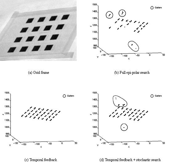
Figure 1: Planar grid sequence


To evaluate the performance of temporal feedback, and analyse the benefit it provides over our standard technique, a series of experiments has been performed. In these experiments different configurations of the SC algorithm have been used to analyse sequences of stereo image pairs;
In the first experiments planar data in the form of our calibration grid was analysed as it rotated about the vertical image axis, figure 1(a) . The planar nature of this data made it possible to perform a quantitative analysis of the performance of the stereo matcher. In the second series of experiments three more complex scenes were analysed: a series of blocks, a toy train and a spider plant, figures 4(a) , 4(b) and 4(c) respectively. In the absence of an underlying model for this data the analysis for these scenes remains subjective.

Figure 1:
Planar grid sequence
A sequence of stereo images, ( ), were taken of the rotating grid. However, the analysis was performed
on a reflected sequence (
 ) derived from the captured images. Analysing the data in forward and
then in reverse served to validate the results and highlight possible
trends in the different configurations. A high degree of self similarity
was another characteristic that influenced the choice of this data. The
images in figure
1
show three re-projections of the final frames from each of the three
algorithmic configurations.
`Outlier' points were automatically identified by comparing the distances of the points to a plane previously fitted to the data. Points more than 5 standard deviations from the plane are marked as outliers. Such outliers are the result of mismatching and may therefore, be used as a measure of matching performance. For each of the three algorithms the number of outliers recovered has been plotted against the amount of data recovered, figure 2(a) , 2(b) and 2(c) . The resulting plot depicts a frame based trajectory of each of the algorithms in `measurement-outlier' space.
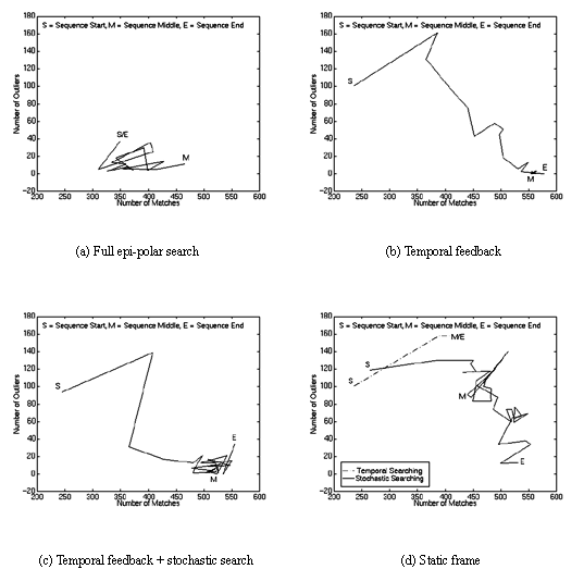
Figure 2:
Trajectory plots for grid data
As figure
1(b)
demonstrates, ambiguity became a problem as a result of full epi-polar
searching. Large quantities of potential matches were rejected by the
global constraints because of inconsistencies. The remaining outlying
edges have been retained by the global constraints because all of the
mismatched blocks in these regions were self-supporting. In figure
2(a)
the trajectory for full epi-polar searching remains relatively
localised, as expected for an algorithm processing frames independently.
The basic temporal algorithm, figure
1(c)
, successfully matched all of the blocks resulting in a near complete
match of all edge features, ( ). The temporal algorithm's trajectory in figure
2(b)
illustrates how the propagation of disparities enabled the algorithm to
converge on the correct solution. A comparison between the temporal and
stochastic trajectories reveals that the stochastic algorithm is able to
converge quicker. However, the inclusion of stochastic searches
re-introduces the problems of ambiguity, although to a lesser extent
than for full epi-polar searching which gives rise to the stochastic
result containing some outliers as well as some missing edge features.
On the basis of the above results, the stochastic search appears not only unnecessary but detrimental to overall performance. However, consider the results presented in figures 3 and 2(d) , which were obtained by iterating the temporal and the stochastic algorithms on a single stereo pair. The temporal algorithm quickly converged on the solution shown in figure 3(a) . Whereas the stochastic algorithm was able to converge on the improved solution shown in figure 3(b) although requiring significantly longer to do so. We conclude that the motion present in the original rotating grid sequence provided sufficient perturbations to enable the algorithm to escape from any local minima. Iterating on a single frame removed the motion component, demonstrating the importance of the stochastic search. Interestingly, the standard temporal result in figure 3(a) is consistent with observed behaviour of the human vision system, more commonly known as the wall paper effect.
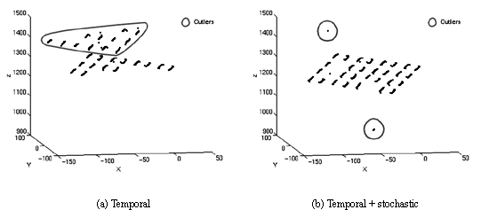
Figure 3:
Planar grid static frame
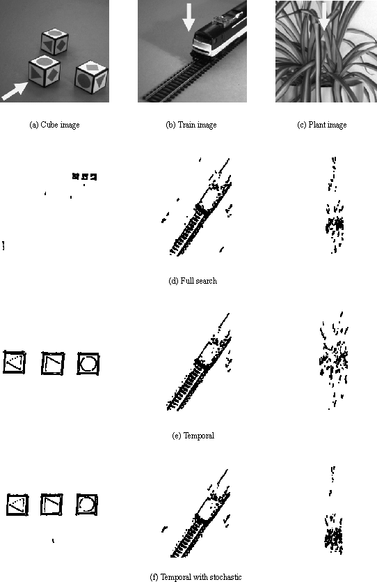
Figure 4:
Scene data examples. Arrows on images show projection direction.
Re-projections scaled to include all outliers.
Although the rotating grid sequence represented a difficult stereo problem, the scenes analysed in figure 4 introduce new complexities; a greater range of disparities, discontinuities, and occlusions. The data presented in figure 4 are re-projections of the 3-D results. Once again, the motions present in the moving cube and train sequences were sufficient to allow the standard temporal algorithm to converge on a result that was preferred to the full epi-polar and stochastic results. Because these far more realistic scenes contained much less self similarity than the original grid images, the full epi-polar search result rejected a lot less data than it did with the rotating grid. However, for the sequence of the train there remained approximately ten mismatched regions in the final result. The stochastic result only contained four small regions of mismatches which compares very favourably with the three mismatched regions in the standard temporal result. However, it is important to note that for the cube sequence the temporal algorithm with stochastic searching did converge on the correct result faster than the standard temporal algorithm.
We have included the spider plant data here as it illustrates a very difficult stereo problem; lots of ambiguity and occlusion. We are currently unable to recover a sensible 3-D interpretation of this scene. Although it is possible to produce far more visually consistent results by enforcing harsher local and global constraints at the block correlation stage, this only succeeds in rejecting large regions of feature data leaving big gaps in the final 3-D result. However, we believe that this kind of scene would benefit from temporal stereo processing due to the increased robustness of reduced search bands as well the enforcement of temporal consistency which should allow these global constraints to be relaxed and hence more correctly matched data to be retained.


Tony Lacey