

To carry out principal component analysis on a data set, we assume that all our data are on a comparable scale. If this is not true, then certain elements of the data set have to be adjusted, in order that incorrect dominance does not occur. However, it is not always immediately clear by how much parameters need to be adjusted in order that the whole data set is on the same scale.
Consider the (standard) shape vector:

Ā

Figure 4:
Ā
(a) The eigenvalues of the shape only model, (b) the eigenvalues as dominates the PCA, and (c) the desired information content as a function
of
Since all points are displacements, they are all comparable with one
another. However, if we add a new value , on a different scale, we might seek a linear factor
 that scales the value of
 relative to the existing
 coordinates:
If , then
 becomes the original shape vector
 , with an unchanged distribution of eigenvalues augmented by zero (such
as in Figure
4
a). As
 , then
 will dominate the PCA with an eigenvalue distribution similar to Figure
4
b, and the information described by the model will tend to zero.
Intuitively, as
 climbs from 0, we might expect the information content of the
eigen-spectrum to rise. At simplest, we might hope for a unimodal
distribution, illustrated in Figure
4
c. We could seek the value of
 that maximises the information measure, thereby optimising the
influence
of the new parameter.
As a suitable measure of the information content of the system, we suggest normalising the eigenvalues:

and then calcultaing the eigen-entropy:

Note that:

and as
as .
.
Using the standard model of flock shape, defined as a shape-only PDM, we
aim to determine the correct scaling of the additional parameters that
were added in section
3
. Letting the additional parameter represent the flock speed, we calculate values of entropy as the scalar
contribution
 of the term
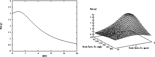
 changes. A plot of the influence of this parameter can be established
(see Figure
5
a), which demonstrates the (ideally) unimodal features of the
information content function we seek. A peak is observed, corresponding
to the value of
 that should be used to scale the additional term
 .
.
Ā

Figure 5:
Ā
(a) A plot of eigen-entropy for different values of , and (b)the
eigen-entropy surface for scaling both speed and velocity angle
simultaneously
The same procedure can be carried out in multiple dimensions by adding in several terms, eg. for velocity angle and robot position, suitable values of the appropriate scalars can be found by maximizing the entropy of the system (see Figure 5 b, for the case of 2 terms).
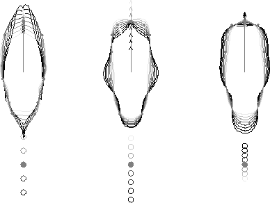
By using these determined scalars in the PDM created in section 3 , we get the improved model seen in Figure 6 .
The principal mode of variation (not illustrated) in the improved model is the same as the first mode of the unscaled model - it concerns the change of flock velocity direction in relation to the robot position. However, the second mode now describes a relationship between the ducks running away faster when the robot predator is closer in proximity. It is also worth noting that the shape change corresponding to this mode is more akin to that of the real animal behaviour; the ducks bunch together when the robot is close, and spread out when the threat is further away.
Thus by maximizing the influence of the additional parameters in the training set, we have extracted the trends in the data that better express the importance of those parameters.
Ā

Figure 6:
Ā
The second, third, and sixth modes of variation of the
correctly scaled PDM flock model.
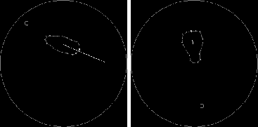
The model so constructed permits the creation of a simulator whose parameters have been derived solely from observed behaviour. For example, under mouse control a robot can be used to pursue a flock of ducks around screen, during which we can observe the flock shape and velocity change according to the relative position of the robot (see Figure 7 ).
At this stage, the simulation is incomplete since it is clear that the behaviour of the animals should be influenced by the proximity of the boundary of the arena in which the pursuit occurs, but the simulation does not mimic this. It is also highly likely that robot velocity (and acceleration) will be influential factors. The approach we have used will generalise to permit these factors to be incorporated when suitable quantities of training data are available.

When we are confident that the model is complete enough to give high quality descriptions of actual behaviour, we will use it as a predictive tool to assist the robot herding strategy that is used in controlling the robotic vehicle. This empirically derived model may also be compared directly with simulations, usually dependent on a small number of (artificial) parameters, to test their validity.


N Sumpter