 be the number of events in bin (
i
,
j
) for the reference histogram and
 the number of events in the same bin in the test histogram.


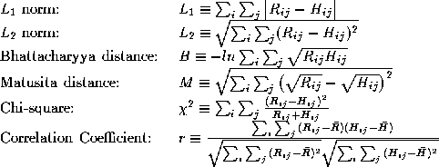
Having created the (chord,angle) histogram of an object we must use it either to identify the object or to characterise the object. One can use the raw histogram directly, or one may try to compute features from it. We shall discuss both approaches. In classification problems we may use one such histogram as the reference one and measure the difference of all other histograms from it. This will result in a single number that characterises the deviation from the reference histogram. Alternatively, if sufficient data are available, the mean histogram for each class can be calculated and the distance of each tested surface from the means of all classes can be found. There are various metrics that have been proposed for histogram comparisons. Those we use in our experiments are defined below:
Let be the number of events in bin (
i
,
j
) for the reference histogram and
 the number of events in the same bin in the test histogram.

In the expression for
r
 is the mean of the
 's and
 is the mean of the
 's.
's.
To improve the sensitivity of the histograms in expressing local
roughness, we must remove from them the component which would be present
anyway, even if the surface we are describing were perfectly smooth. It
can easily be shown that for the surface of a sphere, the relationship
between the angle between the normals and the length
d
of the corresponding chord is:

Although this is a well defined line in the continuous domain, in the
discrete domain it will have some spread, and in order to be able to
subtract it from the histogram of a surface we must calculate the
histogram it gives rise to. In the above expression 2
R
is the diameter of the sphere and at the same time it is the maximum
value of
d
. So, once is specified, a spherical surface with this diameter and with the same
connectivity specifications as our test surfaces is created.
Subsequently, the (chord, angle) histogram of this surface is formed and
is subtracted bin by bin from the test histograms. This may result in
negative bin values. To avoid them we add the same small offset to all
residual bin values, and renormalize the histograms, so each one becomes
again a probability density function. The histograms then can be
compared as described earlier. Alternatively, we may calculate features
from them.
The calculation of features from the histograms is somewhat restricted,
as the first index of a bin is different in nature than the second
index. Therefore, features like contrast and homogeneity cannot be
computed [
6
]. We can only compute the energy and the entropy of each histogram. In
addition, we propose here a new feature, namely the ratio of energies in
the two halves of the histogram corresponding to angles and representing the ``smoother'' characteristics, over the half
corresponding to angles
 and representing the ``rougher'' characteristics:

We call this feature the ``Smoothness'' of the histogram.


Maria Petrou