
In this paper we will present Point Distribution Models (PDMs) constructed from Magnetic Resonance scanned foetal livers and will investigate their use in reconstructing 3D shapes from sparse data, as an aid to volume estimation. A solution of the model to data matching problem will be presented that is based on a hybrid Genetic Algorithm (GA). The GA has amongst its genetic operators, elements that extend the general Iterative Closest Point (ICP) algorithm to include deformable shape parameters. Results from using the GA to estimate volumes from two sparse sampling schemes will be presented. We will show how the algorithm can estimate liver volumes in the range of 10.26 to 28.84 cc with an accuracy of 0.17 ± 4.44% when using only three sections through the liver volume.
Deformable models such as the Point Distribution Model (PDM) have proven to be reliable methods for capturing the statistical variation exhibited in a group of related shapes, and have found many applications in fields such as object recognition and classification [ 1 , 2 ]. One of their most useful characteristics is that they are relatively robust against occlusion, that is, once constructed they can, under certain conditions, still be applied to incomplete data. Thus, as long as the missing data does not completely mask a section of the shape that has the capacity for independent variation, then the models can be used to reliably estimate the shape properties in the region of the missing data.
We have previously shown how the PDM can be used to capture the normal range of variation in 3D shape exhibited in foetal livers [ 3 ], and have exploited its robustness against occlusion to reconstruct liver shapes from limited data where both the spatial orientation of the data in relation to the model, and the point-to-point correspondence between data and model is known. In this work, the utility of the model is further tested by fitting to data where no such prior knowledge of the spatial correspondence between model and data is known. A hybrid Genetic Algorithm (GA) [ 4 ], that incorporates aspects of the Iterative Closest Point (ICP) [ 5 ] algorithm and local shape fitting operators, will be presented as the method of optimising the instantiation of the model from this data. The accuracy of the algorithm in estimating volumes from limited input data using two sub-sampling schemes will be presented.
The PDM is a form of deformable model that has been shown to be a robust method for capturing the variation in shape exhibited by a set of example shapes [ 6 ]. The model is constructed from a number of points, that can be reproducibly located on each example shape. The shapes are then analysed by eigenvector analysis of the covariance matrix formed from the deviations of the point locations from their mean positions [ 7 ]. The eigenvectors are of the form of a list of the deviations in the point locations from their mean positions for each independent mode of variation, and the eigenvalues are the variances associated with each mode of variation, as exhibited in the training set.
The resultant modes of variation, represented by the eigenvectors, form an orthogonal set. We can therefore construct a shape space with each eigenvector representing an axis. If we labelled our shapes with N points in d dimensions, then Nd eigenvectors and their associated eigenvalues are generated giving an Nd -dimensional space, with each dimension having the range of ± infinity. This shape space encompasses all the possible shapes that can be defined with the number of points used. However, not all eigenvectors have statistically significant eigenvalues, so we can reduce the dimensionality of the shape space by rejecting axes corresponding to low significance eigenvalues, keeping only the n most significant eigenvectors. The rejection criteria is usually such that the sum of the eigenvalues of the eigenvectors retained encompass a set percentage of the total variance described by the model - usually 95%, 99% or 99.9%. Furthermore, we can limit the extent of the remaining axes based on their associated eigenvalues. The resultant shape space is now restricted to an n-dimensional hyper-ellipse that describes only those shapes that conform to the "rules" exhibited in the training set. It is this reduced shape space that defines the limits of the search space for the model fitting.
Any of the example shapes, and indeed any shape S contained within the shape space described by the model can now be reconstructed by adding weighted amounts of each eigenvector to the mean shape;
Where S is the mean shape, and w i is the weight applied to the i th eigenvector E i .
The model can therefore be used to fully reconstruct a 3D shape from a limited number of measurements by calculating the values of the weighting factors for each mode of variation that provide the best fit of the model to this limited data. If, as in the general case, neither the spatial orientation of the shape with respect to the model, nor the point-to-point correspondence is known, then an iterative approach to model matching is needed. Firstly, an estimate of the point-to-point correspondence between the given data and the current estimate of shape, initially the mean shape, needs to be found. The next step then finds the best rigid body transformation that superimposes the data points on these estimates of corresponding model points. The final step then adjusts the shape parameters to further minimise the least squares fit of the model to the data. Both of the last two steps will change the estimate of correspondence between the model and the data points, making the current estimate no longer optimal. The process is then repeated to further minimise the model fitting until either i) the root mean square (RMS) distance between the data points and the model points falls below a set threshold, ii) the algorithm converges, or iii) a maximum number of iterations is reached.
The iterative method outlined above will only find a local minima in the search space, and as such a randomised multi-start approach will be necessary to find the global minima. However, if the size and complexity of the search space is sufficiently large, then the algorithm will need to be run for an excessively long time to achieve a realistic probability of finding the global minima. One approach that can be used to better target the sampling of the search space so as to reduce the overall search time is the Genetic Algorithm (GA) [ 4 ].
The GA is a stochastic optimization algorithm that mimics natural evolution. The basic features of a GA are a population of chromosomes -- each representing one estimate of the solution, a means of encoding the degree of freedom parameters of the problem into a chromosome representation, a means of evaluating these chromosomes, a means for choosing chromosomes for reproduction and deletion, and a means of producing new chromosomes. The initial population in a GA is randomly distributed throughout the search space, and the chromosomes are assessed and compared. Chromosomes are then selected for the reproduction process based on how good a solution to the problem they represent. Since the chromosomes of offspring share elements of their parents' genetic material they will be in the same general region of the search space as their parents. In this way regions of the search space that have shown in previous generations to contain near optimal solutions will be searched more thoroughly than less fruitful areas.
We have in this work used a hybrid GA [ 4 ], that retains the overall structure of the traditional GAs, but disposes of the binary representation of the genes and retains a floating point representation. We have also extended the usual range of genetic operators by incorporating reproduction methods that are domain specific, such as local downhill operators including elements of the Iterative Closest Point algorithm [ 5 ] and matrix solutions to the local shape fitting problem.
The motivation for this work is the desire to estimate foetal organ volumes from 3D ultrasound images. For many years foetal weight has been derived from biometric measurements, and used to assess and clinically evaluate pregnancies to improve perinatal outcome. The hypothesis for such studies is that change in organ volume over time will follow some normal growth curve. Abnormal growth, i.e. an organ volume outside the range considered normal for a given stage in pregnancy, may suggest developmental problems requiring a different management strategy. However, there are difficulties with such an approach due to the simplicity of the shape assumptions used and the coarseness of the volume estimation measure.
Ultrasound examination is the usual modality of choice for foetal imaging, but conventional ultrasound is a 2D imaging modality, lacking the positional information necessary for the reconstruction of 3D datasets. A number of methods have been proposed to overcome this limitation, such as 2D phased array transducers or mechanical sector scanning transducers with two degrees of freedom [ 8 ]. An alternate approach is the use of spatial locating devices attached to a standard 2D transducer. These locating devices can be of the form of articulated arms [ 9 ], acoustical ranging systems [ 10 ] or electromagnetic transmitter / receiver pairs [ 11 , 12 ]. The major benefit of the spatial locating device approach is that they can, with appropriate calibration, be used in conjunction with any ultrasound imaging system. Their drawback, however, is that the data acquired is unconstrained, in that the slices are non-parallel, non-uniformly distributed throughout the volume of interest, and may intersect one another at oblique angles. Volumetric measurements of intra-abdominal organs such as liver, spleen and kidney can be estimated using formulae based on ellipsoids and spheres [ 13 ], however the use of these methods is complicated by the nature of the 3D ultrasound datasets, and the accuracy of the results are consequently reduced.
The Medical Physics Department, in conjunction with the Obstetrics and Gynaecology Department at Guy's and St Thomas' Hospitals, have developed a 3D ultrasound imaging system based on a Polhemus 3D locating device attached to a standard ultrasound scanner [ 14 ]. A number of methods have been used to estimate volumes from the images acquired using this system [ 15 ], but to achieve acceptable accuracy a large number of image sections need to be acquired - in the case of the Ultrasound scanned foetal livers, 20 to 30 sections are needed depending on organ size. This relatively large number of image sections presents problems in both data acquisition and analysis.
When acquiring a set of image sections for volumetric analysis it is essential that there is little or no movement of the organ under investigation with respect to the ultrasound probe, since any such movement is not captured by the spatial locating device attached to the probe. This can be difficult to achieve in foetal imaging, because the foetus can move independently of the mother, and is often disturbed by the image acquisition process. An acquisition protocol that requires the capture of only a few images can therefore both greatly reduce the errors introduced by foetal movement, and reduce the amount of interactive data analysis. The aim of this work is to assess whether the use of deformable models can reliably estimate foetal organ volumes from a small number of scans from this system, and to optimise the image acquisition protocol to achieve the optimum accuracy from the number of scans used.
In order to assess the accuracy of the technique for fitting a PDM to limited data, 11 cadaveric foetal livers, chosen from foetuses with normal organ structure and development, were scanned in a Magnetic Resonance (MR) scanner with a voxel resolution of 0.7 x 0.7 x 1.5 mm. This provided a set of evenly sampled, orthogonal slice datasets that allowed the accurate measurement of liver volume and formed a gold standard set of shapes for reconstruction accuracy measurements.
In our earlier work the images were registered to a common coordinate system by identifying three distinct 3D points on each liver [ 3 ]. In this work in order to eliminate any operator error in the choosing of these points, the re-alignment and labelling process was automated. The data was realigned by segmenting the livers from the background by thresholding the images, the data was then translated so that the centre of masses of the liver images were aligned, followed by rotation such that their principal axes were aligned. Next, the data was re-sliced perpendicular to the livers' longest axis to give 25 slices. The surface of the liver on each slice was then found and labelled with ten points equally distributed around the slice contour, giving 250 (x,y,z) triplets for each liver. Liver volumes were calculated using these points by determining the slice area bounded by the slice contour, and multiplying by the slice thickness. A PDM was constructed from all of the data, and an additional 11 PDMs were constructed from subsets of 10 of the example shapes, with each shape being excluded from the model in turn.
Poorly sampled datasets were simulated by re-sampling the original datasets to yield three sections from each shape. Two re-sampling schemes were tested for accuracy of volume estimation and speed of solution. In sampling scheme 1, three slices were selected perpendicular to the longest axis of the liver, with one slice located in the centre of the liver and the remaining slices positioned at approximately an eighth of the way in from each end of the liver. For sampling scheme 2, two slices were selected perpendicular to the long axis as in method one - this time each at approximately a fifth of the way in from each end - with the last section parallel to the long axis approximately central to the liver. Examples of these sampling schemes are shown in Figure 1.

Figure 1. Example datasets showing a) the full data from liver 0, b) the data produced by sampling scheme 1, and c) the data produced from sampling scheme 2.
The PDMs were then used to reconstruct the full shapes from this limited data by finding the best fit of the model built excluding that shape to the three slices. To better simulate the problem that will be encountered when fitting the models to data derived from an ultrasound scanner, the sub-sampled data was then translated and rotated to misalign the data with respect to the PDM's coordinate system, and the GA was then used to fit the model to the data without recourse to the misalignment data or the information concerning which slices were being used. These shape reconstruction tests were carried out fifteen times per liver on each sub-sampling scheme, for each run the data was misaligned in the range ± 5mm in the x and y directions, ± 10mm in the z direction (z being in the direction of the longest axis of the livers), and ± 7.5 degrees about each axis.
An initial population of 200 individuals were randomly generated with x and y translations in the range of ± 10mm, z translations in the range of ± 20mm, rotations about all three axes of ± 10 degrees, and initial guesses for the model based parameters were selected using a Gaussian probability function based of the relevant eigenvalues for that mode of variation. A further 5000 individuals were then generated by the reproduction module, at the end of the run the top 10 individuals were then passed to an iterative downhill operator and the fittest individual was then used to reconstruct the shape.
The objective function is the means of measuring how good a solution to the optimization problem is represented by an individuals genetic material. The measure we wish to minimise is the RMS distance of the data points from their corresponding points on the surface of the instantiated model shape. In our problem the point-to-point correspondence of the data to the model is unknown, in fact for most of the data points there will not be exact equivalent points in the model. We therefore have to find an appropriate distance measure from the data points to the surface of the shape described by the model. This is accomplished for an individual by firstly transforming the data points using the individuals registration degree of freedom values, and then instantiating the model using the shape parameters. Then for each data point: the three nearest model points that form a surface element were found and a plane was fitted to these points, and the perpendicular distance from the data point to this surface was calculated.
The measure of fit between model and data is then the RMS distance of all of the data points to the model. This distance is shown diagrammatically in Figure 2, where A, B, and C are the three model points found closest to the test point D, and d is the distance to be minimised.

Figure 2.
The model (A,B,C) to data (D) distance measure.
The selection of individuals as candidates for reproduction was accomplished in a two step process. First, the objective function for each individual was assessed and the individuals were then ranked in descending order according to this value. Thus the individual with the best measure of fit in the population was given a ranking of 200 and the individual with the poorest measure of fit was ranked 1. Individuals were then selected as parents using the biased roulette wheel method [ 4 ], where the probability P(i) of the i th individual of rank r i being selected is given by:

Once offspring are produced, they are assessed using the objective function and incorporated into the population. Individuals are then selected for deletion by ranking the individuals as above and removing the lowest ranked individuals so as to maintain a population of 200. This method of maintaining the population level is known as steady state replacement [ 4 ].
The usual genetic operators of crossover and mutation used for reproduction in a traditional GA expect and directly manipulate a bit string data format, and as such cannot be used on floating point representations without appropriate modification. The genetic operators used, and their associated percentage chance of being utilised for each reproductive step were as follows:
Uniform Crossover (50%), which is the standard genetic operator from traditional GAs, here we applied it directly to the binary representation of the floating point values as they are stored on the computer; Creep (30%), which uses only one parent individual and each gene has a 50% chance of being perturbed by a random amount; Gene Averaging (10%), in which the offspring genes are generated as the arithmetic average of the parent genes; Point Registration (3%), in which the nearest corresponding points on the surface of the current estimate of shape to the data points were found as shown in figure 2, and the parameters for rotation and translation that provided the best least squares fit registration of the data points to these surface points were found and stored in the relevant offspring genes; Shape Fitting (3%), where the corresponding model points to each data point were found as above and the model weights yielding the best fit of these points to the data were calculated and stored in the relevant genes; Downhill Iteration (2%) which attempts to find a better estimate to the local optimum by iteratively calling the point registration and shape fitting operators. This is, in effect, an extension of the general Iterative Closest Point algorithm [ 5 ] that includes a shape fitting step between each iteration; Random Mutation (2%) in which an entirely new individual is randomly generated.Table 1 shows the relative importance of the first five modes of variation for the PDM created using all of the liver shapes along with the percentage change in volume over the mean shape resulting from the addition of one standard deviation of the first five modes to the mean. It can be seen from this table that the first three modes of variation are associated with the most significant volume changes.
| Mode | Variance | % Variance | %Volume change / SD |
|---|---|---|---|
| 0 | 1230.65 | 31.8 | 29.05 |
| 1 | 906.69 | 23.5 | 14.22 |
| 2 | 632.39 | 16.4 | 14.12 |
| 3 | 448.29 | 11.6 | 0.73 |
| 4 | 219.41 | 5.7 | 1.06 |
Table 1: Relative importance of the modes of variation of the full PDM.
Figure 3, shows the effects of applying ± 2 standard deviations of the first four modes of the model to the mean shape. Mode 0, which accounts for over 31% of the total variance within the model, can be seen to be primarily concerned with describing global scaling of the livers, giving a 29.05% increase in volume over the mean shape for the addition of one standard deviation. Mode 1 primarily describes differential scaling between the two ends of the liver. Mode 2 can be seen to describe a twisting about the long axis of the liver, whilst mode 3 describes a bending along this axis. It is the combination of these modes of variation in varying amounts that allow us to reconstruct a wide range of liver shapes.
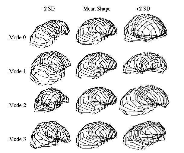
Figure 3. The Effect of standard deviations of the first four modes of variation on the mean shape.
The results from the volume estimation tests are shown in Table 2. The results are reported as the mean and standard deviation of the percentage errors in volume estimation for each liver and sampling scheme, measured over 15 runs for each liver / sampling scheme. For sampling scheme 1, the overall percentage errors in volume estimation were 0.18 ± 6.82% compared with 0.17 ± 4.44% for sampling scheme 2. It should also be noted that in most cases the GA had only just converged on the data from sampling scheme 1 whereas there was little significant improvement in the volume estimation using sampling scheme 2 after 2000 - 3000 individuals. At present each run of the algorithm takes about an 15 minutes to run on a HP 715 / 80 Unix workstation, in order to produce the results presented.
| Shape | Original MR Volume (cc) | %Volume Reconstruction Errors | |
|---|---|---|---|
| Sampling Scheme 1 | Sampling Scheme 2 | ||
| 0 | 10.26 | 2.2 ± 5.3 | -0.3 ± 4.1 |
| 1 | 11.46 | 0.2 ± 5.9 | -2.0 ± 3.5 |
| 2 | 11.67 | 4.7 ± 7.5 | 1.0 ± 2.3 |
| 3 | 16.26 | -4.3 ± 2.1 | 2.7 ± 3.7 |
| 4 | 16.47 | 0.4 ± 4.8 | 2.5 ± 4.7 |
| 5 | 18.40 | 9.7 ± 1.8 | 2.2 ± 3.4 |
| 6 | 18.60 | 2.2 ± 2.0 | 1.1 ± 2.8 |
| 7 | 23.45 | -4.6 ± 3.4 | -4.6 ± 4.3 |
| 8 | 23.71 | -3.5 ± 5.5 | -0.1 ± 1.7 |
| 9 | 26.25 | -7.9 ± 5.2 | 1.0 ± 4.0 |
| 10 | 28.84 | -6.1 ± 3.0 | -1.6 ± 6.5 |
Table 2: Volume estimations from limited data.
This paper has looked at the practicalities of performing multi-variate statistical analysis, in the form of PDMs, on 3D images of foetal livers, and then investigating their use in estimating volumes from limited data. Two different sampling schemes were investigated to help define the best data acquisition protocols for use on the 3D ultrasound system for acquiring data for volume estimation of the organ under investigation.
This study has shown that the algorithms used here can capture the variation in 3D shape exhibited in foetal livers, and can further reconstruct shapes for volume estimation purposes. In addition we have shown that a data acquisition protocol that captures information in more than one orthogonal plane enables the algorithm to converge to a solution both quicker and more reproducibly than acquisition protocols that only acquire data from parallel planes. When using these models on real ultrasound data it should be noted that they will only be used for volume estimation purposes and no other form of diagnosis. What we propose is that the ultrasonographer will perform the usual diagnostic procedures, and only in cases where normal anatomical shape is seen, but organ volume deficiencies are suspected, will data be captured for input to this algorithm. As a further check on the reliability of the estimated volume in each individual case we would propose that a fourth additional image be acquired, which is not input to the algorithm, but compared with the model generated liver contours, which correspond to this region.
The authors would like to thank the EPSRC (grant number GR/K66376), the Special trustees of St. Thomas' Hospital and the Tommy's Campaign for financially supporting this work.
1 . T. F. Cootes, C. J. Taylor, A. Lantis, "Active Shape Models: Evaluation of a Multi-Resolution Method for Improving Image Search", Proc. BMVC 1994, pp 327-336.
2 . T. F. Cootes, C. J. Taylor, D. H. Cooper and J. Graham, "Active Shape Models - Their Training and Application", Computer Vision and Image Understanding, 61, pp 28-59,1995.
3 . C. F. Ruff, A. Bhalerao, S. W. Hughes, T. J. D'Arcy, D. J. Hawkes, "The Point Distribution Model as an Interpolant in the Estimation of Foetal Organ Volume", Proc. CAR `96, Paris, Elsevier, 1996.
4 . L. Davis, "Handbook of genetic algorithms", Van Nostrand Reinhold.
5 . P. J. Besl and N. D. McKay, "A Method for Registration of 3-D Shapes", IEEE Trans. Patt. Anal. Machine Intell. vol. 14, No. 2, pp239-256, 1992.
6 . T. F. Cootes, D. H. Cooper, C. J. Taylor and J. Graham, "A trainable method of parametric shape description", Image and Vision Computing, 10, pp 289-294, (1992).
7 . T. F. Cootes, C. J. Taylor, D. H. Cooper and J. Graham, "Training models of shape from sets of examples", Proc. BMVC., Leeds, Springer Verlag, pp 9-18, (1992).
8 . J. Kisslo, S.W. Smith, O.T. von Ramm, "Real-time, three-dimensional echocardiography: a beginning", Echocardiography: an International Review, J.B. Chambers, M.J. Monaghan, Eds. Oxford: Oxford University Press, 1993, pp.96-101.
9 . R. Pini, E. Monnini, L. Masotti, B. Greppi, M. Gerofolini, "Echocardiographic computed tomography of the heart: Preliminary results.", J Am Coll Cardiol 1989, 49:896.
10 . D. L. King, D. L. King Jr., M. YiCi Shao, "Three-dimensional spatial registration and interactive display of position and orientation of real-time ultrasound images.", J Ultrasound Med 1990, 9:525-532.
11 . T. C. Hodges, P. R. Detmer, D. H. Burns, K. W. Beach, D. E. Strandness Jr., "Ultrasonic three-dimensional reconstruction: In vitro and in vivo volume and area measurement." Ultrasound Med Biol 1994, 20:719-729.
12 . I. M. G. Kelly, J. E. Gardener, W. R. Lees, "3-dimensional fetal ultrasound.", Lancet 1992, 339:1062-1064.
13 . M. J. Zyada, A. R. Jones and P. G. Hogan, "Surface construction from planar contours.", Computing & Graphics, 11, pp 393-408, (1987).
15. S. W. Hughes, T. J. D'Arcy, D. J. Maxwell, J. E. Saunders, C. F. Ruff, W. S. Chiu, R. J. Sheppard, "Application of a new discreet form of Gauss' Theorem for Measuring Volume", Phys. Med. Biol. 41, pp 1809-1821, 1996.14 . S. W. Hughes, T. J. D'Arcy, D. J. Maxwell, W. Chiu, A. Milner, J. E. Saunders, R. J. Sheppard, "Volume estimation from multiplanar 2D ultrasound images using a remote electromagnetic position and orientation sensor.", Ultrasound Med Biol 1996, 22:561-572.
15 . S. W. Hughes, T. J. D'Arcy, D. J. Maxwell, J. E. Saunders, C. F. Ruff, W. S. Chiu, R. J. Sheppard, "Application of a new discreet form of Gauss' Theorem for Measuring Volume", Phys. Med. Biol. 41, pp 1809-1821, 1996.